Dipoles in air and dielectric media (V2D BOR)
The present example considers dipoles in air and dielectric media (V2D BOR).
Axial symmetry allows for performing the antenna analysis with ultra-fast vector 2D Bessel and FDTD hybrid solver (V2D BOR) designated for Bodies of Revolution (BOR) structures. This solver allows for analysing only half of structure's long-section, which results in its extremely fast performance. The structure should be drawn in a way that its symmetry axis coincides with project symmetry axis ρ=0 (in the QW-Editor and QW-Simulator referred as y=0).
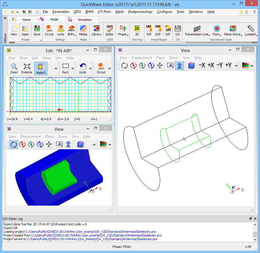
One dipole (V2D BOR) project in QW-Editor.
This example presents radiation by short dipole and small loop antennas. We shall also present a rare feature of QuickWave V2D BOR, which is a possibility to extract radiation patterns in non-air media. Finally, we shall present several power control options, such as checking the balance between power available from the source, power delivered to the antenna, total radiated power, and power radiated through each of the NTF walls.
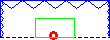
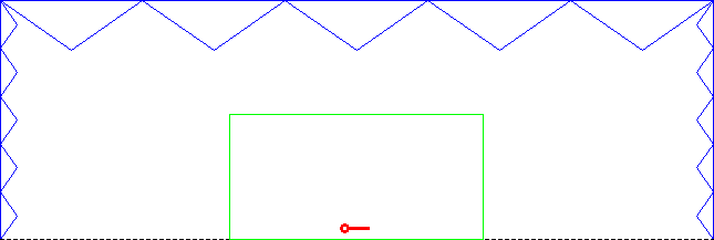
The project concerns a cylindrical volume of space terminated by absorbing walls (blue). A short electric dipole of x-orientation is placed in the vicinity of the symmetry axis (distance of 0.5 mm), inside the NTF surface (green) at which the near-to-far field transformation will be executed for the purpose of calculating the radiation patterns. The angular variation equals 0 thus the dipole represents a small cylindrical radiating surface (a continuous distribution of dipoles on the surface of radius 0.5mm).
Here we shall be analysing ExEρHφ field components, in which case the magnetic symmetry model is appropriate (an electric symmetry model would be appropriate for the dual set of fields, while for non-axially symmetrical modes both models give consistent results).
The exciting field component in this case is Ex, the internal impedance of the source is self adjust for good coupling to the FDTD mesh, and the excitation waveform is pulse of spectrum f<f2 with f2=30 GHz.
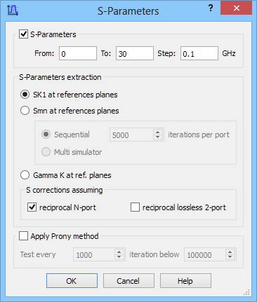
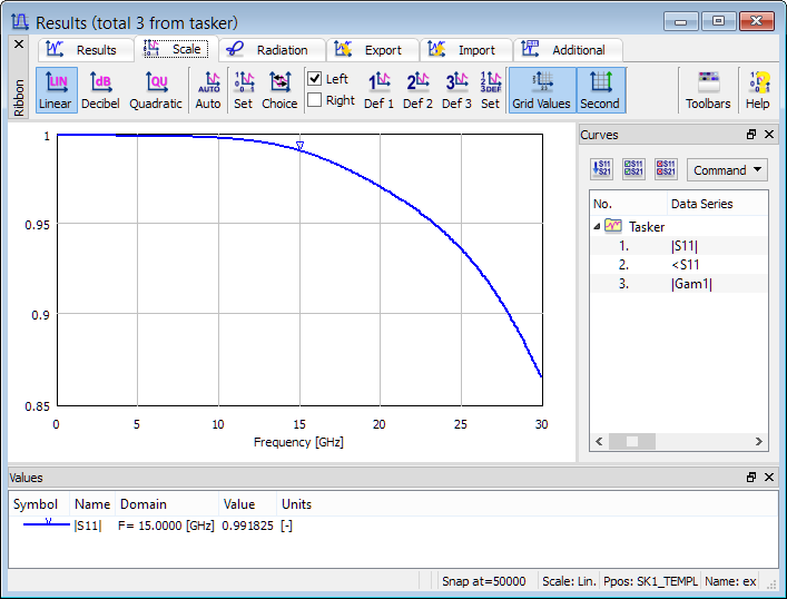
We are interested in obtaining return loss (S11) characteristic and the S-Parameters postprocessing is set from 0 GHz to 30 GHz with the frequency step of 0.1 GHz.
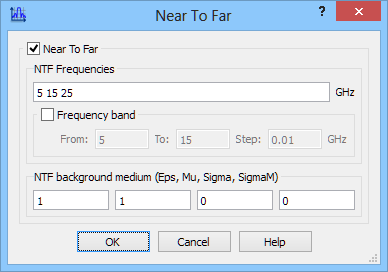
The radiation pattern calculations are activated with Near To Far postprocessing and are set at 5 GHz, 15 GHz and 25 GHz.
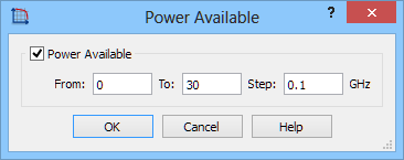
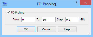
In addition, Power Available and FD-Probing postrpocessings has been activated in the same frequency range as S-Parameters.
S-Parameters postprocessing and Near To Far postprocessing configuration dialogues.
Return loss characteristic.
In addition, Power Available and FD-Probing postrpocessings has been activated in the same frequency range as S-Parameters.
Power Available postprocessing and FD-Postprocessing postprocessing configuration dialogues.
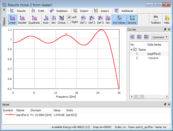
The picture below presents a spectrum of the exciting waveform, which is a square root of time-maximum power available from the source launching this waveform. When configuring the exciting waveform, we have requested a quasi-rectangular spectrum of unit amplitude, dropping to 0.5 at f2=30 GHz. However, the applied pulse duration of 3 periods at the upper frequency has been too short to create this rectangular spectrum, hence leaving ripples. Typically, duration of about 10..30 leads to a rectangular spectrum; however, typically we do not need to have such a rectangular spectrum as the actual value of power available at each frequency can be checked in the Power Available post-processing results.
Power Available postprocessing results.
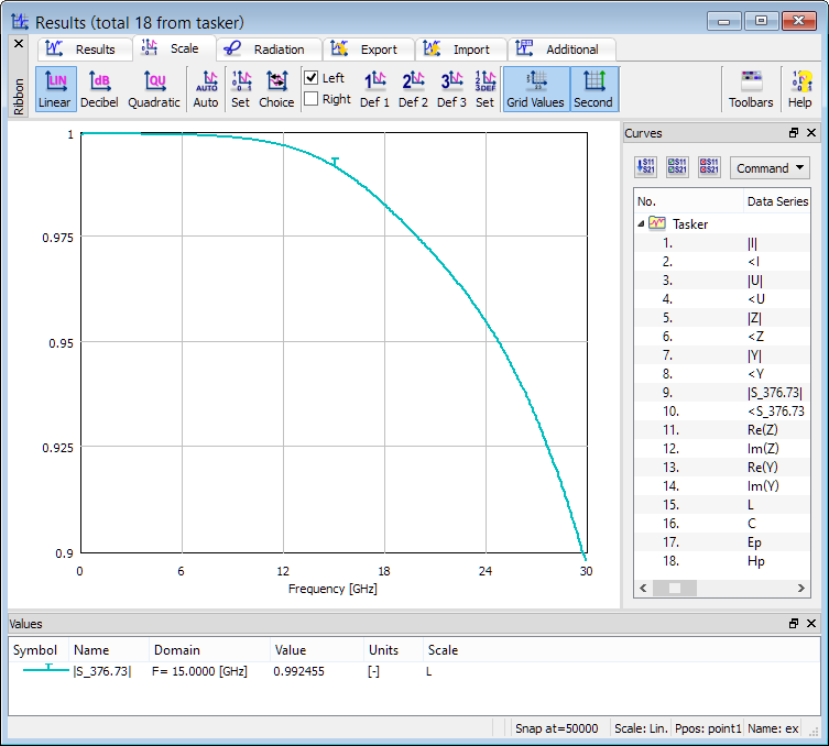
The picture below presents FD-Probing postprocessing results including Fourier transforms of voltage and current at the source and a range of data extracted from there. Note that return loss is provided here (S_376.73) as well as in S-Parameters post-processing but the two values are slightly different: at 15 GHz we get 0.992455 from FD-Probing results and 0.991825 from S-Parameters results. This is because two different current definitions are used in the two post-processing algorithms. In FDTD implementation, lumped electric sources are connected in parallel to the FDTD cell capacitance. The current taken in S-Parameters extraction is a loop integral of magnetic fields around the source; the current taken in FD-Probing postprocessing additionally includes current flowing through the cell capacitance. This distinction has been made to provide additional information.
Return loss characteristic obtained from FD-Probing postprocessing.
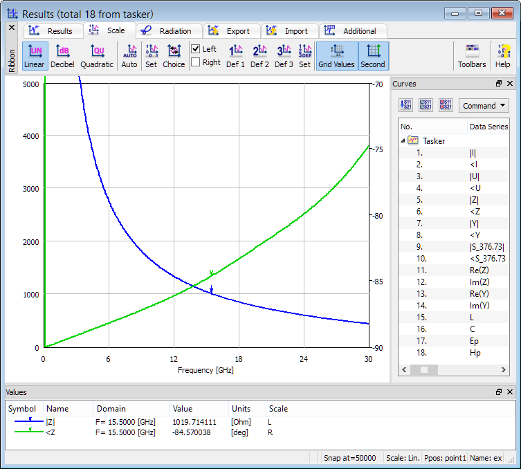
Capacitive character of the impedance is responsible for high reflections. Its magnitude tends to infinity at DC, due to the 1/(fr3) dependence of the dominant electric field component.
Frequency dependent impedance characteristic obtained from FD-Probing postprocessing.
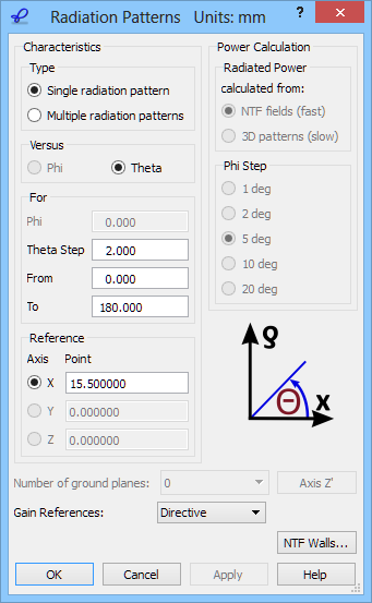
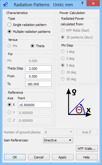
We wish to calculate the 2D radiation patterns versus angle Theta varying between 0 and 180 degrees with a step of 2 degrees. The definition of the angles is explained in the lower right part of the 2D Radiation Patterns configuration dialogue.
The total radiated power can be calculated using two methods, which are directly coupled with the choice of Characteristic Type parameter in Radiation Patterns configuration dialogue. The radiated power (Pr) may be calculated from NTF fields (by integrating the Poynting vector over the NTF surface) and from the 3D patterns in the far zone (for more information refer to Radiated Power online documentation). For horns, rods and other antennas fed by transmission lines both options produce consistent results. In the case of dipoles, the punctual excitation locally violates the divergence law and produces a static spurious mode in the dipole vicinity. This mode does not influence the shape of the radiation patterns or return loss characteristics, but it corrupts the radiated power extraction from NTF fields, especially at low frequencies.
2D Radiation Patterns configuration dialogue with Radiated Power calculated from NTF fields.
2D Radiation Patterns configuration dialogue with Radiated Power calculated from 3D patterns.
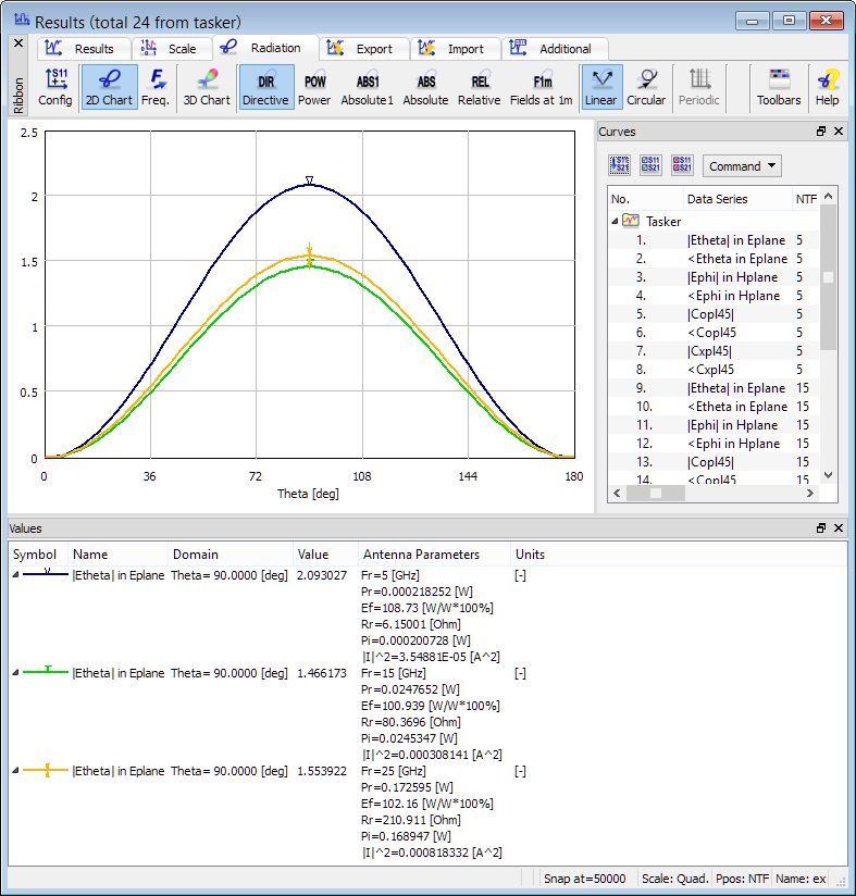
2D radiation patterns calculated at 5 GHz, 15 GHz and 25 GHz with Radiated Power calculated from NTF fields.
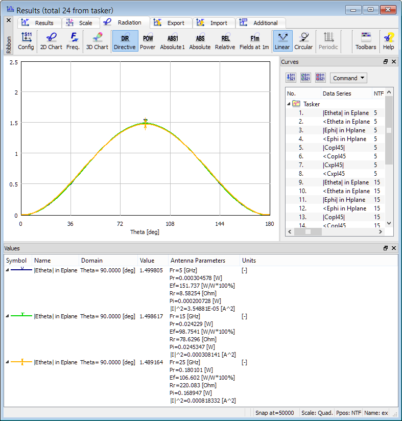
2D radiation patterns calculated at 5 GHz, 15 GHz and 25 GHz with Radiated Power calculated from 3D patterns.
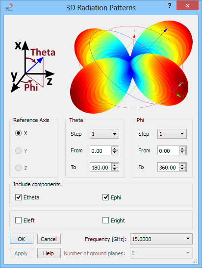
3D radiation pattern, with both Phi and Theta varying in steps, can be calculated in the 3D Radiation Pattern window. The 3D Radiation Patterns dialogue allows setting the reference axis and steps for angles Phi and Theta, defined with respect to that axis in the same way as for the 2D radiation pattern case. A single calculation frequency is also selected.
3D Radiation Patterns configuration dialogue.
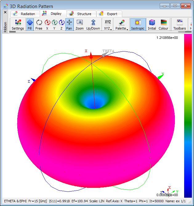
3D radiation pattern calculated at 15 GHz.
Homogeneous media other than air
The near-to-far field transformation is usually applied in air, being the most typical environment for antennas. However, there are cases when transforming near fields to far fields in homogeneous media other than air is of interest. Both QuickWave packages, QuickWave V2D BOR and QuickWave 3D, have been extended in response to such needs. Detailed discussion regarding this functionality is given in Radiation pattern in an arbitrary isotropic medium online documentation.
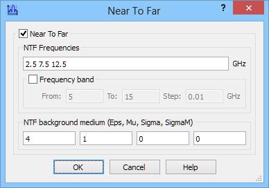
In the second case analysed herein, the space is filled with lossless dielectric medium of relative permittivity 4. To assure effective wave absorption, effective permittivity defined for absorbing boundaries needs to be set to 4. The NTF frequencies have been reduced by a factor of 2 to provide the same resolution of reduced wavelength as in air. Another important case that needs highlighting at this point is that the parameters in NTF Background (Eps, Mu, Sigma, SigmaM) have been set to those of the surrounding medium, namely: 4,1,0,0, to assure accurate calculation of the radiation patterns.
Near To Far postprocessing configuration dialogue.
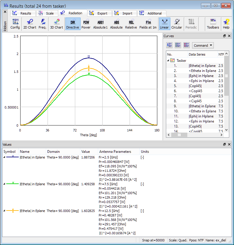
2D radiation patterns calculated at 2.5 GHz, 7.5 GHz and 12.5 GHz with Radiated Power calculated from NTF fields.
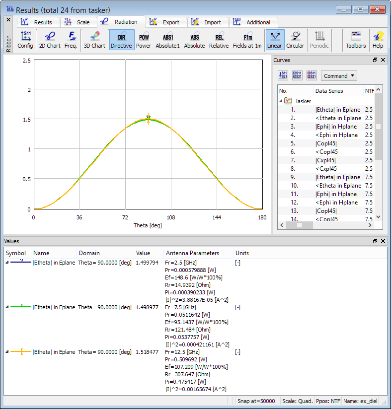
2D radiation patterns calculated at 2.5 GHz, 7.5 GHz and 12.5 GHz with Radiated Power calculated from 3D patterns.
The NTF background medium can also be set as lossy. In such case, the full set of gain scaling options is available only if radiated power is calculated from the 3D patterns in the far zone. Power integration over the NTF box gives a result dependent on the box position and shape, and cannot be used as a reference for scaling the radiated fields. Thus only unscaled values of Fields at 1 m are available in such a case.