3.2.2. Simulation project preparation
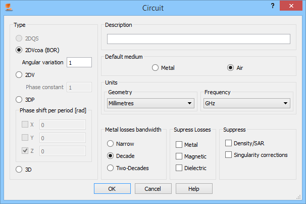
Now, when the UDO script is ready, we can prepare the simulation project. For that purpose we need to run QW-Editor. When QW-Editor is opened, we open Circuit dialogue from Model tab or through Parameters‑>Circuit command in the main menu. In the Circuit dialogue we choose 2DVcoa (BOR) circuit type, denoting axisymetrical structures - two dimensional in cylindrical coordinates. For this type of circuit we need to define proper Angular variation (modal angular variation). In QW-V2D operation, the user has a possibility to excite the structure with the following circular waveguide modes: TMn1, TMn2, TEn1, TEn2. In those names, n is angular variation defined for the project. In case of considered dielectric antenna, we need to excite the structure with TE11 circular mode (determined at the beginning of section 2), thus angular variation must be set to 1 (Fig. 3.2-23).
We must also set the Default medium, which stands for the medium that will surround our structure. In our case the antenna should be surrounded by air thus we make such choice (Fig. 3.2-23).
Fig. 3.2-23. Circuit dialogue with 2DVcoa circuit type chosen.
We now save an empty project as ant3.pro in the directory where the UDO script has been previously saved, using File->Save As option. Then we invoke Draw->UDO Library option available in 2D window. In the window that will appear (as in Fig. 3.2-19) we press Go to->Project button and on the right side of the window the UDO scripts available in the ant3.pro directory will appear. The ant3.udo should be available. We press on that UDO and the Add Object window as in Fig. 3.2-24 will appear (the title bar will also show the path to invoked UDO script). All parameters are correct (the default values defined in UDO header) and we press Draw button. The structure as in Fig. 3.2-25 is drawn. The elements made from metal (waveguide) can be easily noticed since metal medium has a brown colour assigned. Other media that have been introduced to project have default green colour and it is hard to distinguish them. For that reason we will change the colour of two dielectric media that were defined for this project in the UDO script. We do this directly in the QW-Editor and we open Project Media dialogue from Model tab or via Parameters->Media command in the main menu (Fig. 3.2-26). On the right (red arrow) all media defined and available for the project are listed. Name list on the left (green arrow) allows choosing one of those media and editing its parameters. We will edit diel3_6 and diel2_1 media and change their colour.
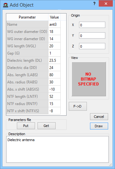
Fig. 3.2-24. Add Object window for ant3.udo.
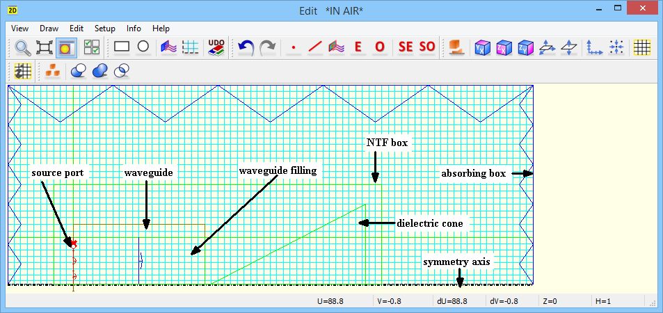
Fig. 3.2-25. Dielectric antenna structure drawn in QW-Editor based on ant3.udo.
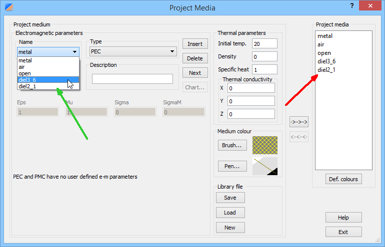
Fig. 3.2-26. Project Media dialogue with project media.
After choosing diel3_6 medium from the list, the Project Media dialogue shows its parameters as in Fig. 3.2-27. We press Pen button and using Color button in Select Pen window we choose brown colour from the available palette. We press OK button in the Select Pen window and perform similar operation using Brush button (this sets the medium colour seen in QW-Simulator Test Mesh option). After setting the colour for Brush, we press arrows button (green frame) to export new medium settings to the project.
Similar operation should be performed for diel2_1 medium (we choose e.g. violet colour). After completing those operations we press Exit button to close the Project Media window. To enforce new media settings we need to redraw the UDO that the project is based on. For that purpose we invoke Edit->Select Object in 2D window. The window as in Fig. 3.2-28 appears. We choose our base udo from the list and double click on it. The window as in Fig. 3.2-24 appears and we press Draw button. The structure will be redrawn with new media settings and will now look as in Fig. 3.2-29.

Fig. 3.2-27. Project Media dialogue for diel3_6 medium.

Fig. 3.2-28. Select Object window.

Fig. 3.2-29. Dielectric antenna structure drawn in QW-Editor based on ant3.udo with new media settings.
Now, when all the elements are well visible we can proceed to the next step, which is setting the excitation parameters.
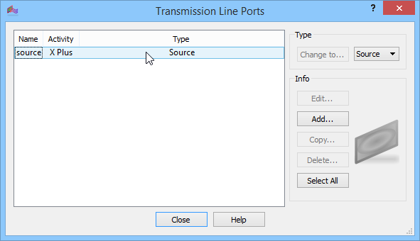
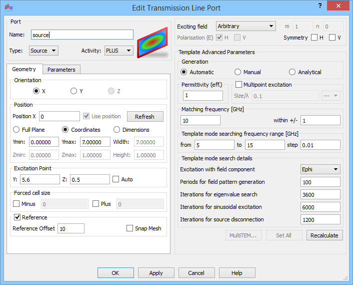
For that purpose we invoke Transmission Line Ports window (Fig. 3.2-30 a) via Transmission Line®Edit Sources and Loads option in Model tab and double click on the source port (Fig. 3.2-30 a) to open its Edit Transmission Line Port dialogue (Fig. 3.2-30 b). We will excite the antenna with pulse excitation in the frequency range from 6 to 20 GHz by choosing pulse of spectrum f1<f<f2 from the Waveform list in the Parameters tab and setting appropriate values for f1 and f2 frequencies. We want to excite the antenna with the circular waveguide mode TE11 and for that purpose we choose Exciting field to be C_TEn1. With angular variation defined as n=1 we get TE11 mode. In the lower right part of the window the exciting filed component should change automatically to be longitudinal magnetic field component Hx and additionally we decrease the number of periods for template mode generation to 60. The above settings are shown in Fig. 3.2-31.
(a)
 (b)
(b)
Fig. 3.2-30. Transmission Line Ports (a) and Edit Transmission Line Port (b) dialogue with default settings.
Now we will put our attention to Template Advanced Parameters frame. We set the Matching frequency (frequency at which the template mode will be generated) to 8 GHz, which is the first frequency from those at which we want the radiation pattern to be calculated. The Template mode searching frequency range will be set to from 6 to 15 GHz (this range should not be too wide so that the template mode can be found at or very close the Matching frequency) with the step of 0.1 GHz. Please note that the effective permittivity Permittivity (eff.) is calculated automatically (assuming air-filled waveguide of radius equal to port height in Y direction) by the software for a given exciting mode and Matching frequency. After changing the value of Matching frequency we need to enforce the permittivity recalculation by choosing once again the Exciting field C_TEn1. We get the value as in Fig. 3.2-32. The negative value of Permittivity (eff.) means that the given Matching frequency is below the cut-off frequency for TE11 mode in air-filled circular waveguide of radius ir. Negative value of effective permittivity prohibits running the simulation. As it has been mentioned above, the software automatically calculates the effective permittivity for air-filled waveguides. In our case we deal with the waveguide filled with dielectric of relative permittivity equal 3.6 and in such cases we need to manually calculate the correct value of effective permittivity and set it in the window. The formula for effective permittivity is given below:
effective permittivity = εr {1-![]() }
}
er- relative permittivity of filling dielectric
fc – cut-off frequency of the mode
f – operating frequency (matching frequency)
In our case cut-off frequency of the TE11 mode in circular waveguide (of radius ir=7mm) filled with dielectric of er=3.6 equals 6.618 GHz. This gives the effective permittivity equal to 1.136. The complete port settings are shown in Fig. 3.2-33.
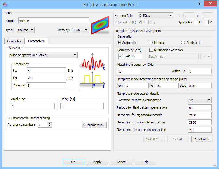
Fig. 3.2-31. Edit Transmission Line Port dialogue with some of port parameters set.
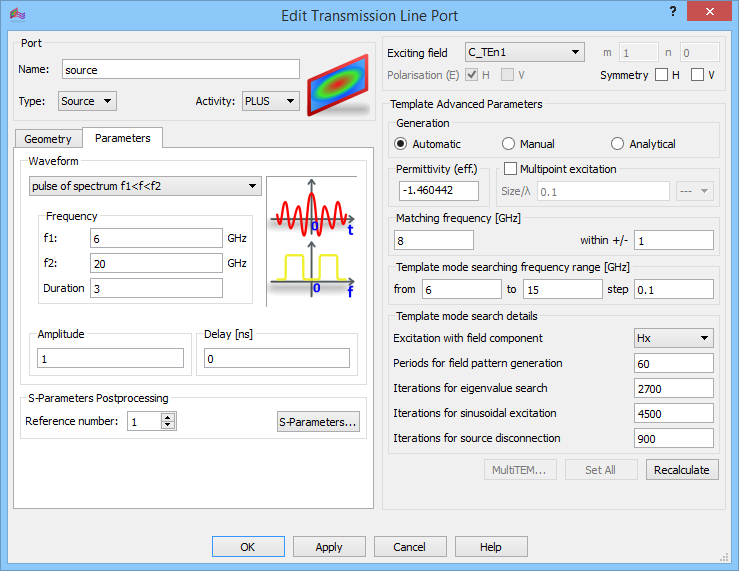
Fig. 3.2-32. Edit Transmission Line Port dialogue with port parameters set.
In general, the port settings are recovered to the default values every time the project is redrawn using Edit->Select Object->Draw, unless in the base UDO script the *.iop file (with port parameters) has been indicated in the port definition CALL command. In our case it was not done while creating the UDO script (Fig. 3.2-18) because we did not have such *.iop file. This will be changed now.
All the port settings that have been defined in Edit Transmission Line Port dialogue can be saved to *.iop file. In the current QuickWave version, the *.iop file can be saved only from I/O Ports Parameters dialogue available under I/O button in Model tab. This is done by pressing Put button. After that, the Save As dialogue appears. Let us put the file name as source and save the source.iop file in the ant3.pro project directory.
Now we shall go back to UDO Editor and ant3.udo file. In the CALL command for exciting port we change the parameter NO to source, as shown in Fig. 3.2-34. This change will cause that whenever the project is redrawn using the UDO script the port settings will be loaded from the source.iop file. It is required now to redraw the project using Edit->Select Object->Draw option to load new port definition. We may save the current version of the project and proceed with setting the mesh parameters.

Fig. 3.2-33. I/O Ports Parameters dialogue with all port parameters set.
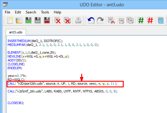
Fig. 3.2-34. Exciting port definition with source.iop file indication.
In case of mesh parameters there are two ways of setting them. We can use manual meshing, where we determine the FDTD cell size that should be enforced. The cell size is determined in each direction separately. When using this meshing procedure we need to remember that when determining the FDTD cell size the following rules should be taken into account:
- We recommend that the FDTD cell size is chosen so that it enables at least 10 cells per wavelength at the highest frequency of interest. Of course there are a lot of cases where the size of the structure comparing to wavelength enforces much denser meshing (when the elements are much smaller than the wavelength and we still need to assure several cells for element’s e.g. height) but it is recommended to not decrease this limit to assure that the FDTD algorithm dispersion error is not bigger than 1.5%.
- The above calculation should take into account the dielectric properties of media present in the project since the wavelength in dielectrics decreases comparing to the wavelength in air.
- If there are metal elements in the project it is recommended to enable singularity corrections for accurate modelling of field singularities near the metal edges, corners, etc. To enable this, all metal edges must be snapped to cell borders. This is done by defining mesh snapping planes at those edges e.g. in UDO script using mesh snapping planes CALL commands (this was done in the original ant3.udo).
In this example we will however use automatic meshing option which may be more convenient for the user. This option is called Amigo (Automatic Meshing Intelligent Generation Option). The advantage of AMIGO is that the user defines the frequency range of analysis and the number of cells per wavelength, and AMIGO enforces the meshing taking into account the materials parameters and introduces mesh snapping planes at all the metal edges and vertexes. It should be noted that AMIGO calculates an appropriate FDTD cell size in all elements (considering their material parameters) and enforces required smaller (compared to cell size in air) cell size only in the regions connected with those elements not in the entire project.
To set the AMIGO parameters we need to open AMIGO dialogue (Fig. 3.2-35) available from Model tab and via Parameters->FDTD Mesh AMIGO command in the main menu. We set the frequency range from 6 to 20 GHz and press Apply button. The Avoid cells below lmin will be highlighted with red thus press arrow button next to this field to recalculate this value and then once again press Apply. We set 15 cells per wavelength and press Apply button, then arrow (to recalculate lmin field) and once again Apply button. The mesh settings in AMIGO dialogue are shown in Fig. 3.2-36. The obtained meshing is shown in Fig. 3.2-37.
The distance between the NTF box and dielectric cone is now 3.5 FDTD cell thus the above condition is obeyed. We save the current version of the project.
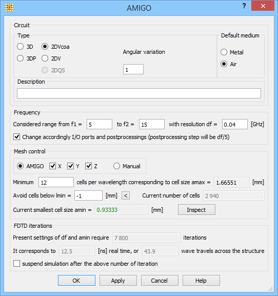
Fig. 3.2-35. AMIGO dialogue with default settings.
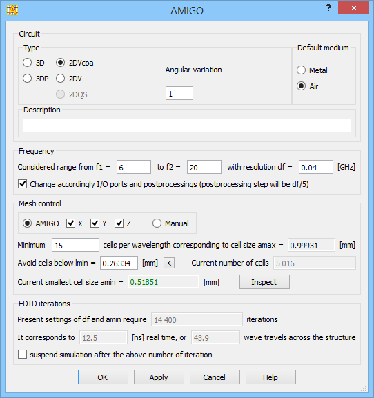
Fig. 3.2-36. Amigo dialogue with mesh settings.
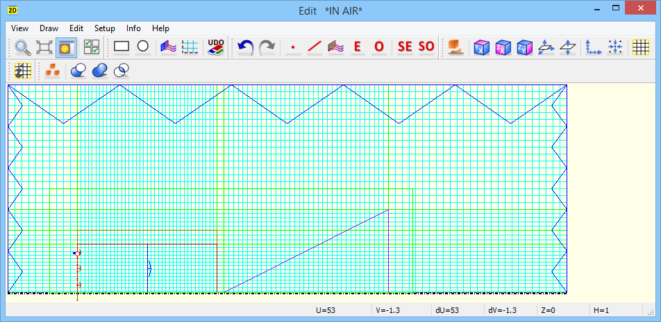
Fig. 3.2-37. Meshing enforced for 12 cells per wavelength setting.
The last stage in preparing the project is defining the post-processings, namely the simulation data that we want to be calculated. As mentioned at the beginning of section 2, we will be interested in reflection coefficient characteristic in 6-20 GHz frequency range and radiation patterns at 8 GHz, 10 GHz, and 12 GHz. For the purpose of activating those post-processings we switch to Simulation tab and open firstly S-Parameters dialogue. We check S-Parameters checkbox for reflection coefficient calculation. The frequency range was transferred from AMIGO dialogue and is correct (from 6 to 20 GHz), we may change the step to 0.01 GHz (Fig. 3.2-38). Secondly, we open NTF dialogue to configure the Near to Far post-processing for radiation patterns calculation. We check Near to Far checkbox and in NTF frequencies we put 8 10 12 (the following values are separated with space). The NTF post-processing configuration is shown in Fig. 3.2-39. The surrounding medium for the antenna is air thus the NTF background medium parameters remain default values.
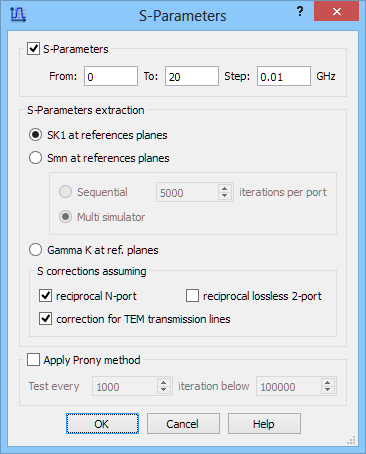
Fig. 3.2-38. S-Parameters dialogue with parameters for S-parameters extraction.
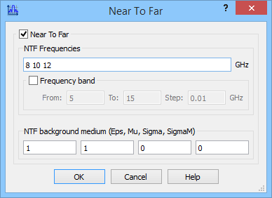
Fig. 3.2-39. Near to Far dialogue with parameters for radiation patterns extraction.
We press OK button and then save the final project. Now we are ready to run the simulation.
We run the simulation with Start button in the Simulation tab. QW-Simulator will be started. We may now watch the reflection coefficient characteristic and radiation pattern results by invoking appropriate results windows available in the Results tab of QW-Simulator (Fig. 3.2-40).

Fig. 3.2-40. Results tab of QW-Simulator.
Please note that the radiation patterns for all three frequencies are available in one window (appropriate curves may be chosen for display from the list on the right side of the window). The simulation results are presented in A dielectric antenna chapter.