2.2 Running the simulations and creating models

The simulations with QProny module can be started from QW-Simulator by selecting an appropriate XXXX_prony.ta3 task file. In fact there are two task files produced by the QW-Editor. One as specified above which contains the preprocessing commands for creating the source templates and the second one XXXX_prony0.ta3, which does not contain the template generating commands. In the case when the simulation is being repeated without any change in the port templates the application of XXXX_prony0.ta3 skips the unnecessary repetition of the template generation.

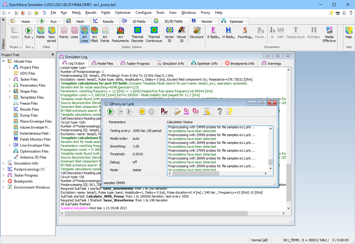
When the Run command is issued on a XXXX_prony.ta3 file from the QW-Simulator menu, the QProny window shown in Fig.P 3.2-1 appears. The central part of the QProny module window shows the calculation status. At start-up the basic simulation parameters are displayed in this part. The most important parameter which should be examined at this stage is the frequency of the energy tests expressed in periods of the central frequency of exciting signal. From equation (P 1-1) it follows that the energy in an RLC circuit decays by the factor e^‑2^{p /Q} per period. Accordingly, the frequency of energy checks, expressed in signal periods, should be greater than 1/5 of the Q-factor of each pole. Too frequent energy checks slow down the simulations and may lead to confusing warning messages and therefore should be avoided. Obviously, the Q-factors of model poles (resonances) are not known a priori but some rough estimates are very often possible. If the value reported in the status window seems to be too low, the simulations should be stopped and the *every parameter in the XXXX_prony.ta3 task file increased. In the example displayed in Fig.P 3.2-1 the tests are carried out every 1000th iteration, which corresponds to about 20 signal periods.

Fig.P 3.2-1 QW-Simulator screen with the QProny module start-up window.

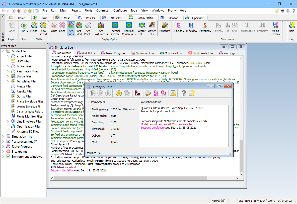
Fig.P 3.2-2QW-Simulator screen with the QProny module window showing warning messages.

As the simulation progresses, the QProny module tests periodically (as configured by the user, see Fig.P 2.3-1) signals at all ports for the energy decay and reports the current status in the central window. The model cannot be created until energy at all the ports starts to decay. If the module detects that there are enough samples to create the model, a set of buttons located on the QProny window tool bar becomes active. Depending on the status of the signal energy either the Yellow Light or Green Light sign lights up. The Yellow Light indicates that while the model can be created, the diagnostics procedures have issued one or more warnings. The text of these warnings is shown in the Calculation Status window (Fig.P 3.2-2). If no problems have been detected, the button with the Green Light becomes active and the Calculation Status window is blank.

In any case, one may press an active light button at this stage. This starts the model creation procedures. Each signal is processed separately and the model orders used are displayed at the bottom status bar of the QProny window. Ideally, all signals should have the same model order. Large variation of the effective model orders usually indicates that the results are unreliable, and a new model should be created when additional samples become available. The creation of the model can be stopped at any point by pressing the Red Light sign in the QProny window button bar.

While the Green Light usually indicates that there are enough signal samples for creating the model, it may happen that the quality of the model is not satisfactory. This may occur especially in complex circuits when signals due to several closely located resonances interfere. On the other hand, simpler circuits can be successfully analysed despite the warnings. Therefore, it is always recommended to create at least two models for different number of signal samples and stop the simulation when they become consistent.