2.7 Fields along user-defined contours - impedance and power extraction
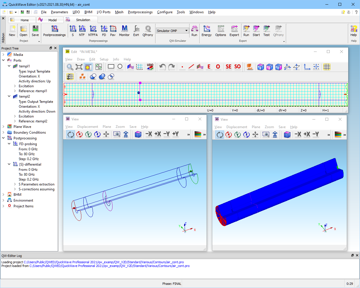
The Various/Contours/water_cont.pro and Various/Contours/air_cont.pro examples are variants of Materials/Dispersive/water_v2d.pro and Materials/Dispersive/air_v2d.pro, respectively. They are supplemented with contours for field integration. The contours have been set with UDO scripts from elib/contours directory and they are visualised in QW-Editor and Test Mesh window of QW-Simulator as in Fig. 2.7-1. Such contours take part in FD-Probing post-processing, which has therefore been added to these projects via FD-Probing dialogue. In QW‑Simulator, an arbitrarily shaped contour is decomposed into segments collinear with electric or magnetic field components. Distribution of these components (Ec and Hc) along the contours can be watched in 1D Fields window. Contributions of line integrals of these components are summed up by the software, producing an integral of the electric or magnetic field along the contour. Time-history of such integrals can also be watched via 1D Fields window, with Uc and Ic components. Finally, the results of space integration are Fourier-transformed by FD-Probing post-processing, similarly as voltages / currents at lumped sources/probes, and accessible via Results window for FD-Probing results.
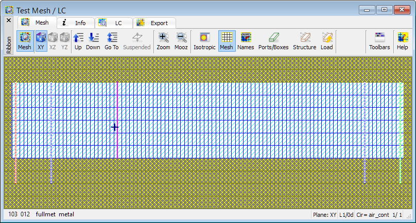
Fig. 2.7-1 Display of electric (magenta) and magnetic (blue) field integration contours in QW-Editor and QW‑Simulator.
In the discussed projects, the electric field contour is a straight radial line linking the inner and outer contours. The result will thus have the physical significance of transmission line voltage. The magnetic field contour is in the φ-direction and of a hypothetical unit length. Consistently with QW‑V2D assumptions, the single Hφ component will be Fourier-transformed and multiplied by 2π, producing the value of transmission line current.
Consider first the Various/Contours/air_cont.pro example, for which the analytically known transmission line impedance is:
Z0 = 376.73* ln(300/75)/(2π) = 83.13 Ω
In QW-Simulator, the ![]() command under
command under ![]() button in Results taballows accessing the results of integration on the two contours in the Results window, see the upper dialogue of Fig. 2.7-2. It is advantageous to highlight both sets (clicking one after the other, with Ctrl key pressed) and to check the Combine Contours option. Then voltage, current and impedance extracted from the two become available in one window, as seen in the Config dialogue on the right of Fig. 2.7-2.
button in Results taballows accessing the results of integration on the two contours in the Results window, see the upper dialogue of Fig. 2.7-2. It is advantageous to highlight both sets (clicking one after the other, with Ctrl key pressed) and to check the Combine Contours option. Then voltage, current and impedance extracted from the two become available in one window, as seen in the Config dialogue on the right of Fig. 2.7-2.
The magnitude of extracted impedance is frequency-independent, as expected, but slightly different from the analytically predicted one (82.56 instead of 83.12 Ω). This is due to the relatively coarse meshing of only 6 cells between the conductors, and the default QW-V2D approximation of fields in the vicinity of the axis, see ref. [42]. These default approximations, called hyperbolic, are optimised to the most typical applications of QW-V2D to horns and cylindrical waveguides; in the case of coaxial circuits, the other set of so-called logarithmic approximations gives better accuracy for coarsely meshed cross-sections of transmission lines. We can switch to the logarithmic approximations by modifying the air_cont.pa3 file, which is one of the intermediate text files between QW-Editor and QW-Simulator.
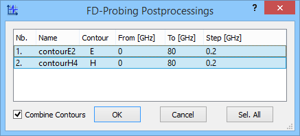
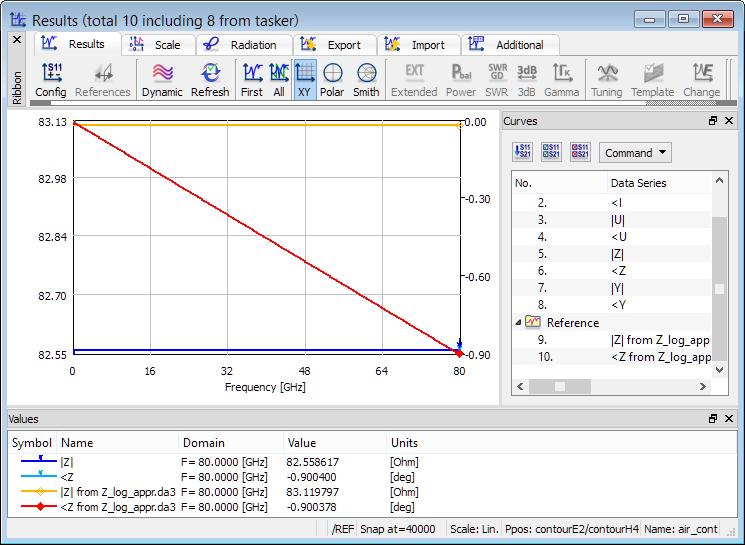
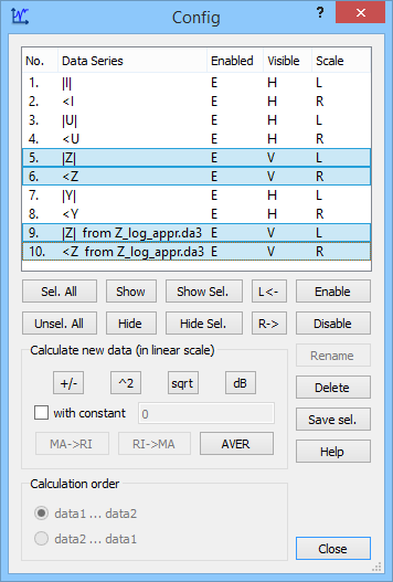
Fig. 2.7-2 QW-Simulator display of FD-Probing results in air_cont.pro example: the dialogue for choosing the set of results, and the results available after Combine Contours.
After locating the file in Contours directory, we modify the line:
2dvcoa 1 *problem type [subtype]
to:
2dvcoa 0 *problem type [subtype]
Stopping the previous simulation ![]() and starting it again with
and starting it again with ![]() , the modified air_cont.pa3 file is used, and Results window for FD-Probing results shows the enhanced impedance result. We have selected both |Z1| and <Z1 in the Config dialogue and saved both in Z_log_appr.da3 file using Save Sel. option. They have been added to the display in Fig. 2.7-2 using Load option in Results window. The precise value of 83.12 Ω is seen.
, the modified air_cont.pa3 file is used, and Results window for FD-Probing results shows the enhanced impedance result. We have selected both |Z1| and <Z1 in the Config dialogue and saved both in Z_log_appr.da3 file using Save Sel. option. They have been added to the display in Fig. 2.7-2 using Load option in Results window. The precise value of 83.12 Ω is seen.
In both simulations (with default hyperbolic and modified logarithmic approximations) the phase of impedance slightly decreases with frequency, down to -0.9˚ at 80 GHz. This results from half-a-cell and half-a-time-step shift between the Hφ and Eρ components on the FDTD mesh, see Fig. 2.7-1. They produce a phase difference between integrated voltage and current by:
0.5(ωΔt - βΔx)
At 80 GHz, taking β from S-parameters post-processing results:
0.5 βΔx = 0.5*1.677mm-1*0.0375mm*180˚/π = 1.8˚
and, due to the stability factor of Δx=2*c*Δt:
0.5ωΔt = 0.9˚
The placement of contours in this project gives partial compensation of phase shifts due to space- and time-shifts to -0.9˚. Moving contourH4 by +37.5 μm in the X-direction (so that it is now placed half-a-cell ahead of the contourE2) causes summation of the two phase-shifts as 0.5(ωΔt + βΔx), leading to 2.7˚ numerical phase of impedance at 80 GHz.
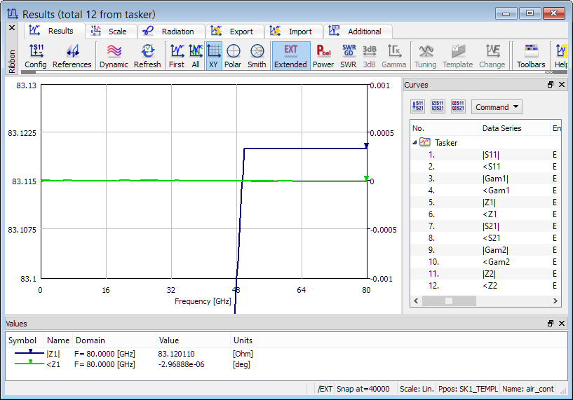
Fig. 2.7-3 QW-Simulator display of impedance extracted in S-Parameters post-processing in air_cont.pro example with modified problem subtype.
Note that impedance is also extracted in S-parameters post-processing of QW-V2D, see Fig. 2.7‑3. In this case, compensation for the time- and space-shifts between the electric and magnetic fields is made within the S-parameters extraction algorithm, and the zero phase of impedance is produced. Absolute value of impedance is obtained as 82.56 Ω (with the default choice of hyperbolic approximations) or 83.12 Ω (Fig. 2.7‑3 snapped after by modifying problem subtype in the air_cont.pa3 file).
Note that the value of impedance produced by both:
- S-parameters post-processing
- FD-Probing post-processing
is constant in frequency and identical to the quasi-static value of impedance displayed by QW-V2D in the Simulator Log window during template generation, since the transmission line is non-dispersive.
Consider now the use of contour mechanisms for validating electromagnetic power levels in the transmission line. As demonstrated in Dipoles in air and dielectric media, time-maximum of power available from the source can be obtained via Power Available post-processing. The Contours/air_cont_P.pro is a variant of the original Contours/air_cont.pro, to which the Power Available post-processing has been activated in QW-Editor. Moreover, Breakpoints in QW-Simulator have been configured to suspend the simulation after 2000 iterations (this instruction is stored in Contours/air_cont_P.br3 file). Launch the air_cont_P.pro example from QW-Editor using ![]() button, and the simulation will be automatically suspended after 2000 iterations.
button, and the simulation will be automatically suspended after 2000 iterations.
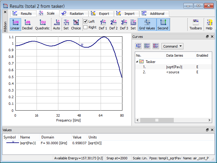
Fig. 2.7-4 QW-Simulator display of power available from the source in air_cont_P.pro.
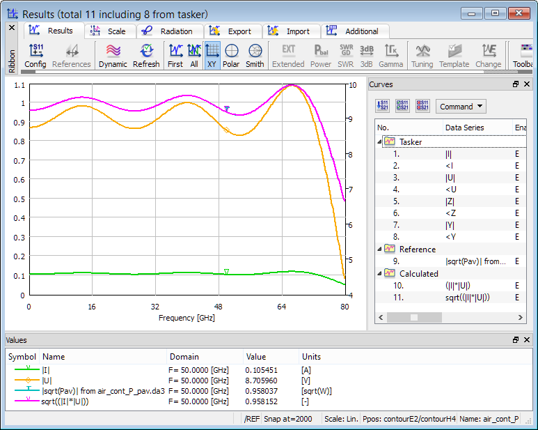
Use  button to open Results window with Power Available post-processing results as in Fig. 2.7-4. The |sqrt(Pav)| characteristic is square root of time-maximum of power available from the source versus frequency. In the settings of QW-Editor, we have requested a quasi-rectangular spectrum of unit amplitude, dropping to 0.5 at f2=80 GHz. However, the applied pulse duration of 3 periods at the upper frequency has been too short to create this rectangular spectrum, and we get ripples within ±10% of the unity. Typically, duration of about 10..30 leads to a rectangular spectrum; however, typically we do not need to have such a rectangular spectrum as the actual value of power available at each frequency can be checked in the Power Available post-processing.
To see the results of Power Available post-processing together with FD-Probing post-processing results in one window, we need to save |sqrt(Pav)| characteristic to a file, and then add it to the FD-Probing results display. For that purpose Save sel. option of Config dialogue is used, and the |sqrt(Pav)|curve is saved to sqrtPav.da3 file.
Fig. 2.7-5 QW-Simulator display of current, voltage and square root of their product obtained from FD-Probing on contours, and square root of power available from the source previously saved to sqrtPav.da3 file, in air_cont_P.pro.
Open another Results window with FD-Probing resultsshowing |I| and |U| curves and Load sqrtPav.da3 file. In the Config dialogue perform multiplication operation to get (|I|*|U|) curve, which has the significance of amplitude of power flowing in the transmission line. To make it commensurate with the previously loaded square root of available power, calculate sqrt((|I|*|U|)) curve and press ![]() to display the new curve. The navy blue curve will be added to the window (see Fig. 2.7-5). The two curves coincide what confirms that, for the matched transmission line, power flowing in the line and calculated from contours equals to power available from the source and calculated by Power Available post-processing.
to display the new curve. The navy blue curve will be added to the window (see Fig. 2.7-5). The two curves coincide what confirms that, for the matched transmission line, power flowing in the line and calculated from contours equals to power available from the source and calculated by Power Available post-processing.
Consider now the same project but with sinusoidal excitation at 50 GHz - air_cont_P_sin.pro.
Invoke 1D Fields window as in Fig. 2.7-6, which shows the Uc component being the time-dependent integral of the electric field along contourE2. This is the same quantity as has been Fourier-transformed and shown in Fig. 2.7-5. As given in the upper window in Fig. 2.7-6, the 1D Fields window will show 400 recent time samples, and no samples will be automatically saved (Save time scale is 0).
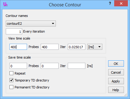
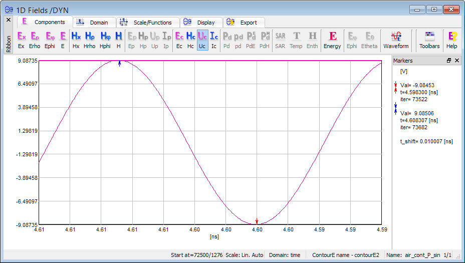
Fig. 2.7-6 QW-Simulator display of voltage integrated along contourE2 versus time (lower picture), with settings as in the upper picture, in air_cont_P_sin.pro.
Invoke another 1D Fields window, which will show the Ic component, as in Fig. 2.7-7. In both Fig. 2.7-6 and Fig. 2.7-7 we have Domain: time (window status bar), which means that the horizontal axis is time. Note that the axis is oriented from right to left (samples towards the left are at more recent time instants). The two windows have be opened at different moments (Start at: 72500 and 72877 iteration, respectively) and hence up to the current 73776 iteration they have been active for 1276 and 899 iterations, respectively, as also shown in their status. Nevertheless, they show samples of voltage and current, respectively, for the same recent 400 time steps. Time-maxima of voltage and current occur at the same moment (iteration 73682, corresponding to time 4.608307 ns) and so do the minima (iteration 73522, corresponding to time 4.598300 ns) since we have a pure travelling wave and the two contours are at only half-a-cell distance. As discussed previously in this Section, this leads to half-time-step separation between the integrated voltage and current. We may also verify that the period of excitation equal twice the time-shift between maximum and minimum is correctly 1/(50 GHz) = 0.02 ns.
The amplitudes of Uc and Ic shown in Fig. 2.7-6 and Fig. 2.7-7 are approximately 9.085 and 0.110, respectively. These are higher by a factor of 0.958 than the values of approximately 8.706 and 0.105 depicted in the cursor pane of Fig. 2.7-5. This is because the sinusoidal excitation of unit amplitude used now provides the available power of 1 W, while the pulse excitation used in the previous experiment provided a smaller available power of (0.958)2 =0.918 W at 50 GHz.
If the Dynamic mode of the window is turned off, the samples are still assembled and the set of last 400 ones will be shown upon window redraw (or keyboard space).
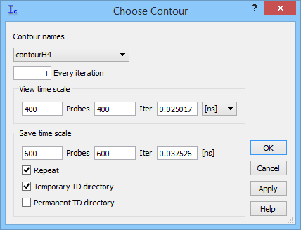
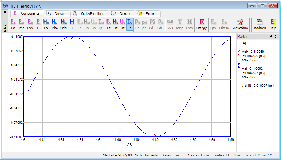
Fig. 2.7-7 QW-Simulator display of current integrated along contourH4 versus time (lower picture), with settings as in the upper picture, in air_cont_P_sin.pro.
The settings of Fig. 2.7-7 indicate a non-zero Save time scale of 600 iterations. This means that from the moment the window is opened, the 600 samples of Ic will be assembled and saved to air_cont_P_sin.tpd file in Temporary TD directory created within the project directory. The name of the sub-directory is built of project name, contour name, component name, and date of creation. e.g.:
air_cont_P_sin_contourH4_Ipoint_Mon Feb 25 11_25_41 2014
Since the Repeat option is checked in Fig. 2.7-7, consecutive sets of 600 samples will be saved in consecutive air_cont_P_sin files with tpd1, tpd2,… extensions. This means that a history longer than the dynamically monitored 400 samples will be available for inspection. The Fields®Saved 1D Fields command of the main menu should be used to this end, and one of the tpd files should be selected. The Setup-Switch-Change View Iterations commands allow adding previous or consecutive file contents to the same window. Fig. 2.7-8 shows an assembly of samples from three consecutive files.
Since Temporary TD directory option is selected in Fig. 2.7-7, the directory (and all its files) will be deleted from disk when the 1D Fields window (which has created this directory) is closed. If the user wishes to maintain the history, the Permanent TD directory option should be selected in Fig. 2.7-7 instead. Note that the Temporary TD directory option is the default one, since *.tpd text files accumulated during a long simulation may occupy vast disk space.
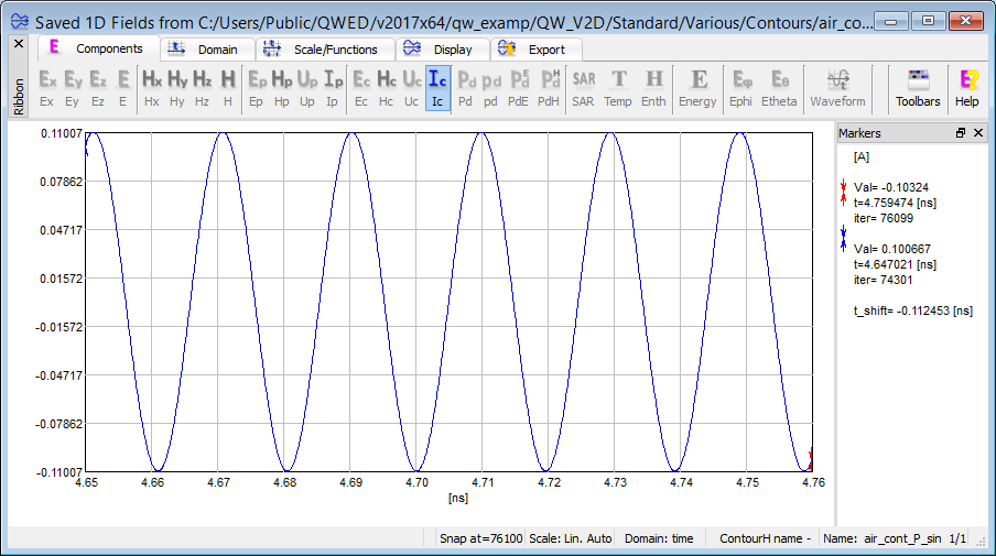
Fig. 2.7-8 QW-Simulator display of current integrated along contourH4 versus time obtained in the Saved 1D Fields window with loaded on three previously saved tpd files.
Besides monitoring the integrated voltages and currents, it is also possible to monitor electric or magnetic field distribution along contours. The left picture of Fig. 2.7-9 shows another 1D Fields window, with Ec component selected. We now see Domain: contour (window status bar), which means that the horizontal axis is along the considered contourE2. Note that Ec (like all electric field components in QuickWave) is divided by a square root of intrinsic impedance of vacuum and expressed in the electric field units of [V/mm]. The previously considered Uc (or U in FD-Probing results) is an integrated quantity in [V], and not scaled by the impedance of vacuum. Summing up the values along the Ec envelope, multiplying by cell size 0.0375 mm (constant along radius), and multiplying by sqrt(376.73..) restores the value of Uc amplitude of 9.085 V.
Since contourE2 in this example is a straight line in the radial direction, the display of radial electric field along the Y axis (denoting the radial axis in QW-V2D) should be identical. Such a display is generated by another 1D Fields window (Domain-Space-Y Axis set at X=29 (the contour is along the left edge of 29th cell in the horizontal direction, see Test Mesh window), and Erho component). The resulting display (right in Fig. 2.7-9) is indeed identical with the contour display along the contour, extended with zero fields beyond the contour (inside the conductors).
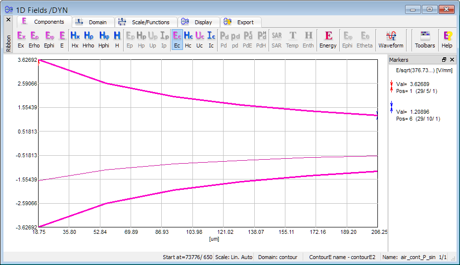
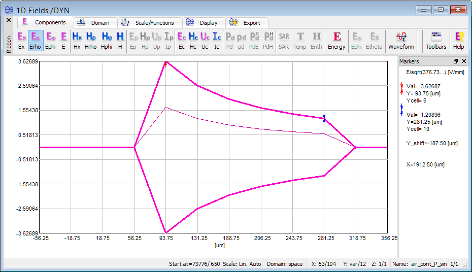
Fig. 2.7-9 QW-Simulator display of electric field along contourE2 and radial electric field along the Y (rho) axis.
After invoking two 2D/3D Fields Distribution windows (with Fields button) we get the display as in Fig. 2.7-10 showing instantaneous distribution of the radial electric field in two xρ planes. The two patterns are identical due to axial symmetry of the TEM mode. The maximum value of the field at the inner conductor (3.627 in QW scaling for electric fields) is equal to the previously noted in Fig. 2.7-9. The right window shows the angular magnetic field in one xρ and one ρφ plane. Due to the QuickWave scaling of electric fields divided and magnetic fields multiplied by a square root of vacuum intrinsic impedance, the amplitudes of Eρ and Hφ H in this air-filled TEM line are identical.
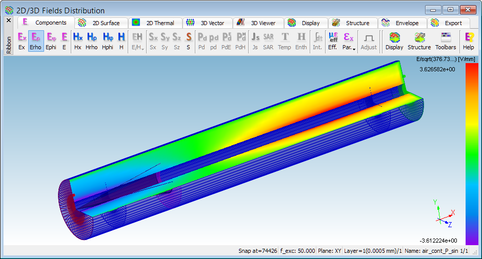
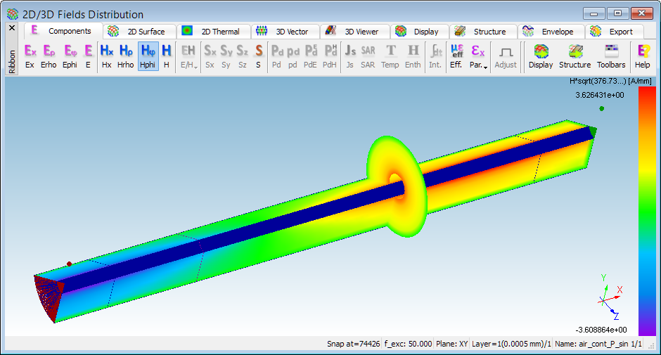
Fig. 2.7-10 Art Filled display of radial electric field in two xρ planes and angular magnetic field in one xρ and one ρφ plane.
Fig. 2.7-11 appears in response to invoking another 2D/3D Fields Distribution window and shows the Poynting vector in thermal display. The maximum value of 13.15 [W/mm2] is noted at the inner radius and is consistently equal to the product of the electric and magnetic field amplitudes (3.627)2.
In many practical examples, the Poynting vector appears most informative in vector display. Here due to coarse meshing of the cross-section of the line this display is poorly visible. In Fig. 2.7-11 it has been snapped in a zoomed mode and with the structure display removed
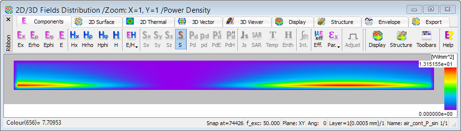
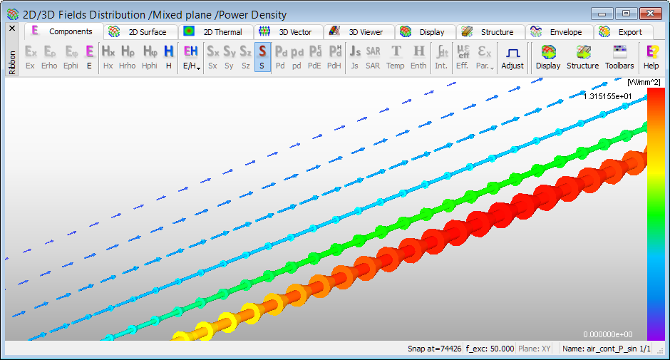
Fig. 2.7-11 Thermal and Vector display of Poynting vector.
The above displays of Poynting vector are scaled as power flux density in [W/mm2], centred at the location angular magnetic field. In some cases, it may be informative to watch them scaled as power flux through a ring spanning the 2π angle, and extending by ± half radial cell size from the centre Hφ node. This is obtained via V2D Plane (Shift+G) option, which invokes the upper dialogue of Fig. 2.7-12. Choosing the power flux through a ring option produces the lower display in the same figure. Note that the maximum value has changed from 13.15 in Fig. 2.7-11 to 0.2905 in Fig. 2.7-12, which consistently equals: 1.315*10*2*p*(37.5*10-3)2*2.5.
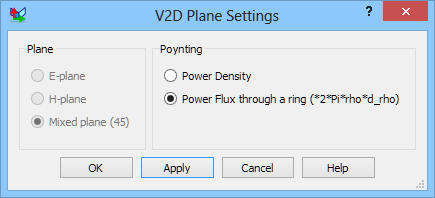
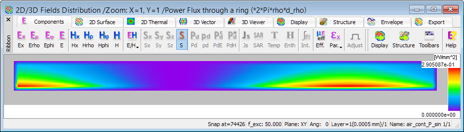
Fig. 2.7-12 A dialogue for switching between the displays of power flux density and flux through a ring and the display obtained in the latter case.