1.1         Specific aspects of FDTD analysis in QW-V2D

Fundamentals of the FDTD method of analysis have been discussed in Fundamentals of the Method of Analysis. In Introduction to QW-V2D package it has been signalled that QW-V2D is applicable to the structures of axial symmetry (also called Bodies of Revolution or BOR). In such a case, the 3D electromagnetic problem reduces to two dimensions in cylindrical coordinates xr and the FDTD method reduces to a 2-dimensional (2D) one. In general, we can distinguish scalar 2D problems with only three non-zero field components, or more complicated vector 2D problems (V2D problems) in which we must consider all six field components. As suggested by its name, QW-V2D can deal with vector 2D problems, but the analysis of simpler scalar 2D problems is also possible. 

The FDTD method requires that the structure under consideration be divided into cells. In the classical 2D FDTD method the cells are rectangular. The modified conformal FDTD method applied in QW‑V2D software package allows much more flexibility of the FDTD cell shape. This will be explained later in this Chapter.

The QW-V2D package consists of two main programs: QW-Editor and QW-Simulator. QW‑Editor plays a double role of a graphical editor, which allows the user to define his problem, and a conformal mesh generator, which automatically performs the meshing process. The conformal cells created by QW-Editor are exported to QW-Simulator.

There are two important consequences of using the vector two-dimensional formulation of FDTD in cylindrical coordinates:

·       Firstly, QW-Editor generates only one layer of cells.

·       Secondly, this layer corresponds to the xrhalf-plane, above the axis of symmetry, which is pre-defined at r=0 (y=0).

The first observation entails that in the V2D regime, only a long-section of the structure in the xr-plane is considered. No elements, objects or ports may extend below the axis (into the r<0 half-plane). Since the physical structure is known to be axisymmetrical, the notions such as “level” or “height” along the j–direction are irrelevant. However, purely for compatibility with the 3D regime of QW‑Editor, we define all elements at a fictitious level = 0 and of fictitious height = 1. The only exception is NTF (Near to Far transformation) box, automatically created form ntf_2dv.udo at level = 0.25 and of fictitious height = 0.5. These fixed fictitious values cannot (and should not) be modified by the user.

A well-known problem of the cylindrical coordinates is that some of the field components become singular at the axis of rotation, and cannot be obtained with the standard FDTD equations. In QW‑V2D, a remarkably simple and accurate treatment of these axial singularities has been implemented. The basic idea is to snap to the axis those components, which are either known to be identically zero, or are unneeded for updating of any other fields. This leads to two models of the axis:

·       as an electric symmetry plane (PEC boundary, short) passing through the line of E_jE_x H_rfields;

·       as a magnetic symmetry plane (PMC boundary, open) passing through the line of H_jH_x E_rfields.

It can be proven that for non-axisymmetrial modes (n>0), both models of the axis are admissible and produce consistent results. For axisymmetrical modes (n=0), the choice of the model is uniquely determined by wave polarisation. In the TE_j case (comprising the H_j E_x E_r fields) a magnetic symmetry plane must be used at the axis. In the TM_j case (comprising the E_j H_x H_r fields) an electric symmetry plane must be used at the axis.

In the classical FDTD all the cells would be rectangular. In the conformal FDTD method applied in QW-V2D they can be of a shape of a rectangle or a rectangle cut by an arbitrarily passing straight line. This means that the cells adopt a boundary conforming shape, which can precisely model the boundary which is curved, inclined or composed of steps smaller than the cell size.

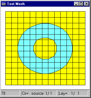
As an example, Fig. 1.6-1 compares the conformal model generated by QW-V2D and a classical stair-case model of a toroidal resonator, constructed as a loop of the 50 W coaxial line. The difference between the two meshes is apparent. Despite rather coarse discretisation the conformal mesh of QW‑V2D well preserves the circular shape. The stair-case mesh converts the outer conductor into a Manhattan-style structure and the inner conductor into a square.

Fig. 1.6-1. Meshing of a toroidal resonator, constructed as a loop of the coaxial line (inner/outer radii of the line 1.521 mm/3.5 mm, basic cell size a=0.8 mm, yellow – metal, blue - air): conformal mesh generated by QW‑V2D (left) versus classical stair-case mesh (right). Both displays are zoomed – the axis of rotation is five cells below the visible area.

Fig. 1.6-2 shows conformal meshing of a horn antenna, with shallow opening of the horn. The conformal mesh well preserves the sloped boundary, and will support the correct surface currents. The stair-case mesh prolongs the input waveguide feed, and replaces the actual horn with stepped straight waveguide sections. This will deviate the physical path of current flow, leading to spurious peaks or nulls in radiation and scattering patterns.

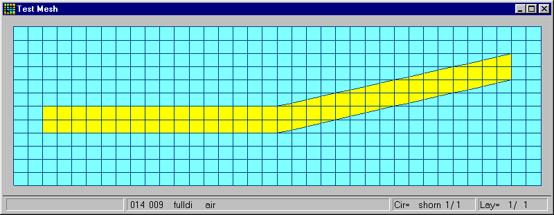
Fig.1.6-2 Meshing of a simple horn antenna, with shallow opening (yellow – metal, blue – air): conformal mesh generated by QW-V2D versus classical stair-case mesh.

Although both above examples have been concerned with curved and oblique metal boundaries, the meshing process is accomplished in the same way in the case of any media interfaces, for example, a boundary between two dielectrics. QW-Editor always approximates the physical structure with a set of cells, where each cell can be filled with two different media separated by a plane. QW-Simulator, through its internal conformal geometry compiler, converts this cell-by-cell description into matrices of auxiliary local electromagnetic parameters.

The meshing strategy outlined so far provides competitive accuracy in representing volumetric variations of materials. However, it would not be sufficiently accurate for problems involving strong field singularities, for example, near metal corners, edges, and thin wires. Therefore QW-Editor additionally allows the user to define thin metal wires (of diameter specified by the user, and smaller than the FDTD cell size). The mesh generator automatically adds information about the presence of these special elements to the description of appropriate cells. The conformal geometry compiler of QW-Simulator takes into account these wires, and also the automatically detected right-angle metal corners, by introducing special corrections for field singularities.

The following general remarks should be summarised:

·       The conformal model often produces very small cells (see for example Fig. 1.6-1or Fig. 1.6-2). Contrary to the classical FDTD algorithms, in QW-V2D these boundary-matching cells do not cause any stability problems and do not require time-step reduction. This is because the small cells are internally merged to the neighbouring cells.

·       QW-V2Dassumes singular field behaviour around wires. To enable singularity corrections at the edges and corners of metal blocks, the user should ensure that respective edges coincide with the mesh (e.g., by setting mesh snapping planes). All singularity corrections in the whole circuit can be suppressed by the user through the Export Options of QW-Editor.

·       The shape defined by the user (in the QW-Editor) is built of basic elements like a house is built of bricks. The basic types of elements are rectangles and polygons; a polygon of sufficiently many sides accurately approximates a circle (Fig. 1.6-3).

·       The shape can also be defined using objects, which are automatically decomposed into elements by QW-Editor.

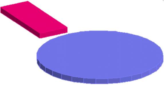
Fig. 1.6-3 Typical elements of QW-Editor: a rectangle and a 32-side polygon approximating a circle.

·       There are two types of objects. The first one concerns internal objects, which are simply groups of elements, and/or other objects put together for easier execution of common operations like for example a shift to another position. The other type concerns external objects, which are groups of elements produced externally. Typical way of creating external objects is by means of a UDO script. Such objects can be easily modified from their headers. Select Object  command opens the list of objects used in the project. They are marked as udo or normal. Mouse double click over a udo object opens its header and enables modification of its parameters. Note that an object defined by a UDO script but called internally from another UDO script is marked here as normal, and not udo, because its header is not accessible from that level.

·       UDO scripts are grouped in libraries placed in the installation tree as subdirectories of “elib”. Invoking Draw-UDO Library  opens the list of objects available in the current library. Left click over an item opens its header while a right click opens a menu enabling access to the object description and to the udo script for its possible modification.

·       An alternative way of geometry definition resides in importing CAD formats. It is possible to read *.dxf files. Pressing DXF button in the Model tab makes it possible to read a dxf file and convert it to a UDO script, which is then immediately run. The UDO object obtained from DXF Converter appears on the list of objects  and can be modified or deleted from there. To obtain correct results, we must have a dxf file describing a polygon (not an open broken line) and without internal subroutines sometimes used in ACAD. DXF projects with subroutines must be first read, “exploded” in ACAD software and saved again before they can be read by DXF Converter.

·       The axis of rotation is pre-defined at r=0 (y=0).The axis becomes visible if any element, object or port has been defined.

·       No elements, objects or ports may extend below the axis (into the r<0 half-plane).

·       Assign the correct mesh snapping properties to the axis of rotation.An electric symmetry plane must be placed at the axis for the analysis of axisymmetrical TMjmodes. A magnetic symmetry plane must be placed at the axis for the analysis of axisymmetrical TEjmodes. Either of the two can be used at the axis for the analysis of non-axisymmetrical modes.