2.9.1       A circular waveguide junction

We will start the discussion of biphased objects by considering the example wgjun1.pro. It has been created by a single call to ct2r.udo of the library junctions, with the following set of parameters: 30, 22, 40, air, Y, 2, 180. The example has been recorded in the DRAFT phase of QW-Editor obtained by pressing  under  button in Modeltab of QW-Editor. Let us note that all the biphased objects are supposed to be drawn (and later possibly modified) in the DRAFT phase. Then the phase should be changed to FINAL by pressing  before the project is exported to QW-Simulator.

a) 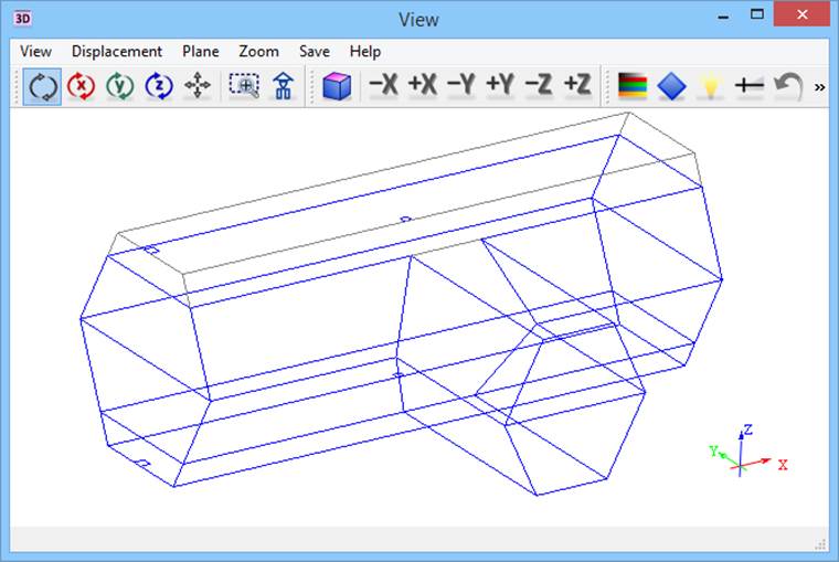 b)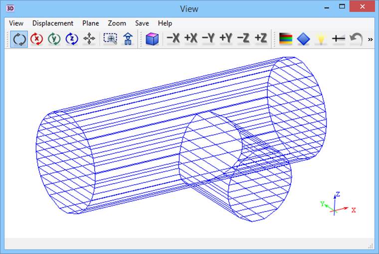

c)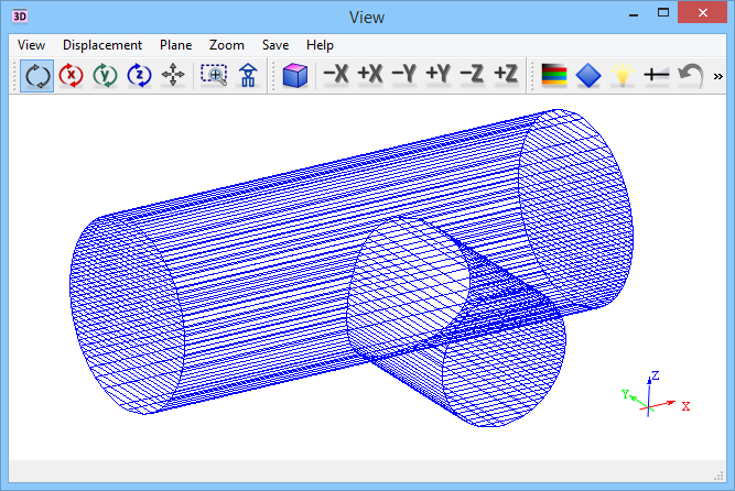

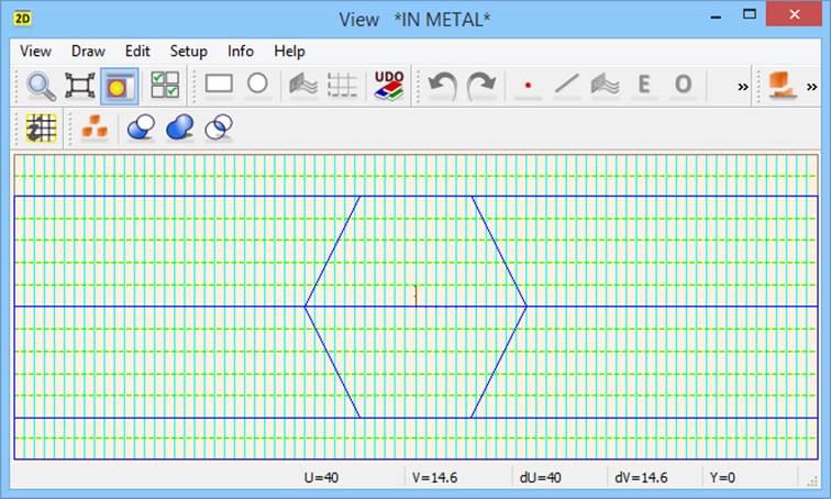
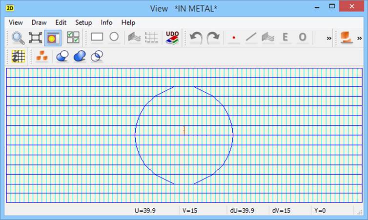
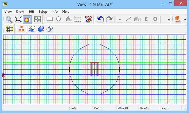
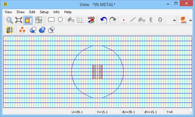
Fig. 2.9.1-1 Views of wgjun1.pro example in one 2D window in XZ-plane and one 3D window: a) in the DRAFT phase with Z-axis mesh of 5 mm (upper left) b) in the FINAL phase with Z-axis mesh of 5 mm (upper right) c) in the FINAL phase with Z-axis mesh changed to 2 mm in the preceding DRAFT phase (lower).

Let us look at the image of wgjun1.pro in the DRAFT phase, as shown in Fig. 2.9.1-1a. The considered circular waveguide junction is represented very roughly. In fact, only its location is marked, and its approximate shape is outlined. We can also see that a relatively coarse mesh of 5 mm has been chosen in the Z-direction.

Now let us press . Upon this command the software will redraw all the biphased objects of the current project in their FINAL phase. It will try to make the best geometrical approximation of these objects possible on the mesh defined in the preceding DRAFT phase. In other words, it produces mesh-adaptive slicing of the object creating a separate combined element at each sublayer of the FDTD cells. The result is visible in Fig. 2.9.1-1b.

Let us note that in the last DRAFT phase we have applied a coarse mesh of 5 mm along the Z-axis, which entails that the height of each FDTD sublayers cannot exceed 2.5 mm. That is why the FINAL phase produces the object sliced into 14 prisms. We can verify the number and height of prisms moving the cursor in 2D Window in XZ-plane (using Zoom option may be convenient) or by  command (it shows the Select Element list with 28 entries because both bottom and cover of each prism are recorded).

In the FINAL phase we can refine the FDTD meshing, for example to 2 mm. However, please consult the  list to see that the number and height of prisms have not changed. Although each prism has been resolved into several FDTD sublayers (as in Fig.2.9.1-2d), the shapes of the prisms has not changed, and the curvature of the cylinder walls will not be better approximated.

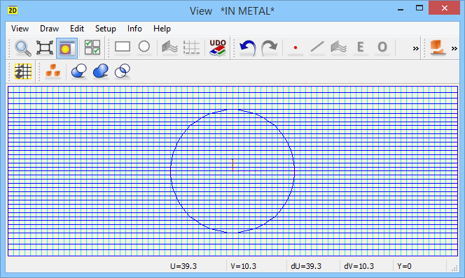
If we want to improve the curved boundary approximation, we must adapt the slicing to the finer mesh. We return to DRAFT phase, set the meshing (for example to 2 mm), and call the FINAL phase again. As a result we obtain a precise approximation of the cylindrical structure presented in Fig. 2.9.1‑1cand Fig. 2.9.1-2c. Note that Fig. 2.9.1-2shows zoomed displays of 2D Windows in XZ-plane.

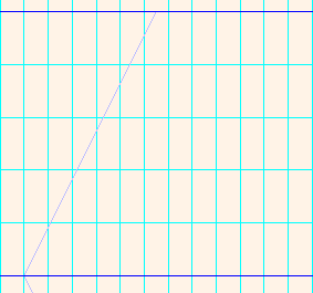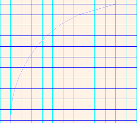a)   b)   c)   d)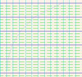

Fig. 2.9.1-2 Approximation of biphased elements curvature by prisms. Cases a, b, c correspond to a, b, c of Fig. 2.9.1-1; case d) has been produced from b)  by refining the Z-mesh in the FINAL phase (c).

This example illustrates the first advantage of the application of the biphased objects:

·       Biphased objects permit to adjust the approximation of the surfaces curved in the Z-direction precisely to the applied meshing.

Note that “the applied meshing” concerns not only mesh resolution set by the user, but also mesh snapping planes possibly enforced by other objects. In particular, when modelling metal insets with sharp edges or corners, it is advisable to snap the mesh to their surfaces in order to improve the modelling of field singularities.

Let us consider a metal matching post added to the considered wgjun1.pro. We will first perform an incorrect operation of adding the post in the FINAL phase. We press , go to the basic library, and select cyvo.udo object with parameters: cyv1,2,6,16,metal,E,0,0,-3. The parameter E indicates that mesh snapping planes will be set at the bottom and top of the post. We obtain a display recorded in wgjun1b.pro and shown in Fig. 2.9.1-3a. The mesh snapping planes of the post are offset by just 0.8 mm from the previously constructed slice of the waveguide junction, which produces a very thin sublayer. By putting a red dot on the left of the 2D Window, QW-Editor warns us about this thin layer and expected slow-down of calculations, and suggests reconsidering our geometry definition. The red dot is shown when the local cell size is less than 0.3 of the standard cell size for the particular coordinate direction (as declared in Mesh Parameters dialogue).

While keeping the mesh snapping planes of the post can be important for overall accuracy, there are no arguments against adjusting the definitions of cylindrical surfaces to the modified mesh. We press  (to come back to DRAFT phase and thus eliminate the previously constructed slices) and then  (to produce new slices), and obtain a display of Fig. 2.9.1-3b. The final meshing is significantly more uniform, and the red dot has disappeared.

a)  b) 

Fig. 2.9.1-3 Meshing of the wgjun1b.pro obtained after adding a metal post in the FINAL phase of wgjun1.pro, and an improved more uniform mesh created after going through DRAFT and FINAL phase. 

Adjustment of slicing to the mesh is not the only advantage of biphased objects. Note that we often need to compose a complicated structure from various library objects. Imagine that such objects are sliced into layers independently. In such a case it may happen that the limits of slices of different objects fall accidentally very close (but not identical) to one another. This will produce a very thin layer of FDTD cells. To maintain the algorithm stability under such circumstances, the software will reduce the time step and the computing time would rise inversely proportionally to this time step.

Such a situation can be avoided when we use biphase objects and thus:

·       Mesh adaptive properties of biphased objects allow synchronised slicing of all objects of the project. Consequently, we obtain slicing with the smallest possible variations of the height of individual slices, which results in important savings in the computing time.

As it has been pointed out in FDTD method in QuickWave Software, QW-Editor internally operates on elements (simple or combined). In general, the elements are composed of polygonal bottom and cover and linking edges (or in short links). Elements are supposed to have the same number of vertices in the bottom and the cover, and uniquely defined links between them.  Whenever we perform Boolean operations on objects (Edit-Join-Cut/Join/Intersect), the elements belonging to one object enter into Boolean operations with the elements of the other object. It is quite clear that in the class of combined elements the Boolean operations (like Cut or Join) may produce the cover with a different number of vertices than the bottom. Thus the software needs to make intelligent decisions about connecting the vertices. However, often there is no unique “the best” solution and thus even a sophisticated algorithm may produce rather unintuitive or even unreasonable distribution of the links.

The distribution of links in elements is important if we want to perform further slicing of these elements into layers and sublayers of FDTD cells. In such a case the links decide about the shapes of intermediate sublayers.

However, when the element height is reduced to just one FDTD sublayer, the links become practically irrelevant. They may somewhat perturb the displays of QW-Editor, but do not influence further electromagnetic analysis by QW-Simulator. This is because the mesh interpretation algorithm of QW‑Simulator analyses the shapes of sublayer bottom and cover, and draws the conclusions about its side walls without referring to links.

Easy decomposition into single-sublayer elements is facilitated by biphased objects. Therefore:

·       Biphased objects can automatically adjust the elements to the cell size and produce the elements of a single FDTD sublayers height. This enhances the accuracy of geometrical approximation of the objects obtained after Boolean operations on the original objects.

More discussion of the Boolean operation on objects will be given in Boolean operations on elements and objects of this manual.