2.5.2       Rectangular waveguide filter

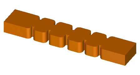
We will consider a waveguide filter proposed by P.Ibbs and M.Guglielmi in the September 1996 issue of Microwave Engineering Europe. Fig. 2.5.2-1 shows a general external view of the filter. It is built in a 19.50 x 9.525 mm rectangular waveguide. Dimensions of resonators and irises will be specified further, but note that the irises are symmetric and span full height of the waveguide.

Fig. 2.5.2-1 A general view of the considered waveguide filter.

Let us remark that formally speaking, this filter analysis belongs to the category of the S-Parameters extraction problems. Therefore, the user is recommended to first read S-parameters extraction problemsof this manual, which provides a detailed discussion of various co-processing and post-processing options applicable in such a case. Nevertheless, the tutorial of the present Section does not assume this earlier knowledge. It describes how to use the functions of QW-Editor and QW‑Simulator appropriate for this example. It also depicts several specific aspects such as the use of symmetry conditions and metal loss modelling. 

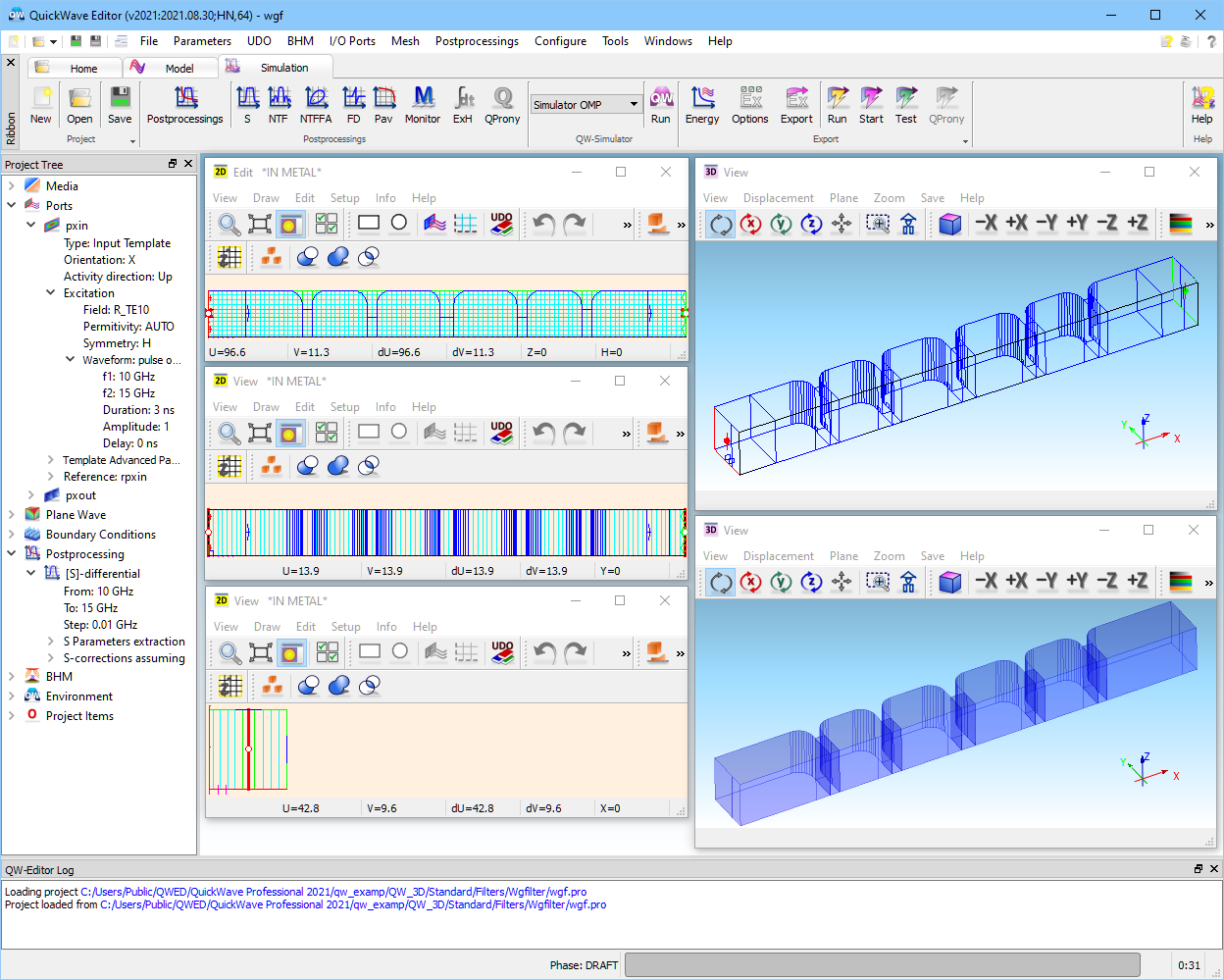
Fig. 2.5.2-2 A screen of QW-Editor with loaded wgf.pro.

The geometry and simulation parameters for the filter are stored in wgf.pro file. Please open QW‑Editor, click over  button, and browse the example directories to find and load ..\Filters\Wgfilter\wgf.pro. Fig. 2.5.2-2 shows the image, which will appear on your screen. This is the main window of QW-Editor, as indicated in its title bar. The title bar also shows (in brackets) version number and date; the "H1" symbol stands for the type of the appropriate hardware key. Following the dash is the name of the project.

We will now formulate introductory remarks on understanding the displays of QW-Editor. The readers interested directly in the FDTD simulation process and results may skip one sub-section and proceed to "Running QW-Simulator".

Interpreting QW-Editor displays

Below the title bar we can see the list of main menu commands and Ribbon tabs. Those applicable to the present example will be explained throughout this Section, while a complete overview is given in User Interface of QW-Editor.

The filter is visualised in five windows: three 2D Windows (left), two 3D. The 2D Windows, from top to bottom, show structure cross-sections in the XY–, XZ -, and YZ –planes. In general, the user can open as many of such windows as needed for clear display, but at least one 2D Window in XY–plane is necessary for drawing and modifying the geometry.

We immediately see that only half of the structure has been defined and will be analysed. This is possible due to the already noted symmetry condition. Since the filter will be excited with the fundamental TE10 mode, we consider a magnetic symmetry plane (PMC – perfect magnetic conductor) along the X-axis. This plane is graphically shown as a dark framed rectangle (in the 3D Window and 2D Window in YZ-plane) or a dark line (in 2D Window in XY-plane).

Note that we can also define and analyse the full filter. In fact, this would be necessary if we wanted to investigate the effects of technological asymmetries. However, by taking advantage of the magnetic symmetry condition, we are reducing the required memory and computing time by a factor of two.

Furthermore, note that we have defined the interior of the filter. In other words, we have drawn the volume of air filling input and output waveguides, resonators, and coupling slots. Since a default colour for air is blue, the 3D Window solid view shows a blue solid block, and the other windows – blue contours of air elements.

What remains to be explained is how metal boundaries (PEC – perfect electric conductor) have been set along the top, bottom, and side surfaces of the filter. This brings us to the very important notions of default medium and default external boundary.

A default medium is a medium automatically occupying all regions of the project, which have not been explicitly filled with any other medium. We may imagine that our project definition starts with an infinite space of default medium. We then place geometrical elements, sources, and loads inside this space. The FDTD mesh is created over a region defined by outermost dimensions of these elements, sources, and loads. Only in this region the FDTD simulation is subsequently performed.

Irrespectively of our choice of the default medium, the default external boundaries for the FDTD mesh are PEC. Therefore, in this wgf project, whatever default medium we choose, the top and bottom walls will be PEC. PEC will also be placed along the outer side wall of waveguides and irises, although the inner volume of irises will be filled with the default medium.

QW-Editor offers two choices of default media: metal and air. A default medium chosen for a particular project is signalled in title bars of all 2D Windows. For wgf we read *IN METAL*, which means that metal occupies all space outside the blue block shown in 3D Window solid view. This explains why we do not have to define explicitly the material of irises.

External boundaries other than PEC have to be set explicitly, irrespectively of the default medium. The definition of PMC symmetry plane has already been mentioned. Furthermore, the input of the filter will be excited by the input port (source) marked as a red rectangle with three arrows, while the output is terminated with an absorbing load marked as a green rectangle.

S-Parameters will be extracted between the reference planes associated with the source and load, and marked as blue rectangles, each with a single arrow. The band of excitation and post-processing is 10..15 GHz.

As a final step before running the FDTD analysis, let us take a look at the constructed mesh. In the XY-plane the cell size of approximately 1 mm has been applied. This ensures 20 cells per wavelength at the highest frequency of interest, and also resolves the width of each iris into no less than 2 cells. On the other hand, the height of the filter is modelled with just one 10 mm cell (note that the XZ-and YZ-plane windows show two half-cells, corresponding to the two sublayers, as introduced in FDTD Method in QuickWave Software). This is possible because along the Z-axis there is no variation of the modelled geometry and no variation of the considered TE10 mode pattern. Thus, our problem is effectively two-dimensional. There will be no field variation and no wave propagation in the Z-direction, and hence the mesh in this direction is restricted neither by wavelength nor geometry resolution.

Running QW-Simulator

To start the FDTD analysis from QW-Editor, please click over  button from Simulation tab. QW-Editor will export (save on disk) a set of files describing the geometry and parameters of simulation, then it will call QW-Simulator, and QW-Simulator will start the analysis.

The main window of QW-Simulator will show up, as in Fig. 2.5.2-3. Its status bar includes an iteration counter, refreshed every second. The title bar indicates version, hardware key, and the name of the project. Below we can see the list of main menu commands and Ribbon tabs. Those applicable to the present example will be explained throughout this Section, while a complete overview is given in User Interface of QW-Simulator.

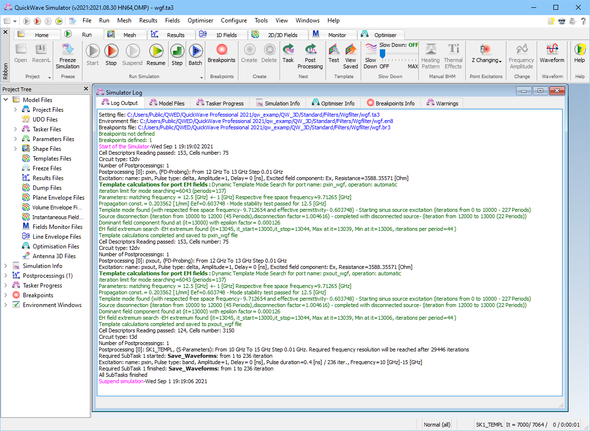
Fig. 2.5.2-3 QW-Simulator main window: upper part and status line at 7000 iteration of wgf analysis.

A major part of display of Fig. 2.5.2-3 is occupied by the Simulator Log window. It records consecutive operations performed by QW-Simulator. After a few introductory lines related to setting the appropriate project-related files, we can see two sections (each starting with Template calculations… and ending with Template calculations completed…), which describe the process of template calculations. Templates are field patterns for the modes assigned to the input and output ports. In our case, both are the fundamental TE10 mode. The details of the template generation process have been discussed in First insight template generation.

The last line in the Log Output tab of Simulator Log window indicates that simulation has been suspended by the user. This has been done by clicking the  button in Run tab of QW-Simulator. Now the FDTD processing remains at iteration 7000. It would continue upon pressing  button.

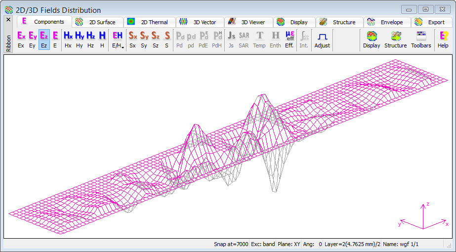
Fig. 2.5.2-4 Vertical electric field at 7000 iteration of wgf analysis – 2D Surface display.

We now invoke 2D/3D Fields Distribution window by pressing  button in 2D/3D Fields tab of QW-Simulator. This brings up window displaying Ez component of electric field in one cross-section of the analysed structure (Fig. 2.5.2-4).

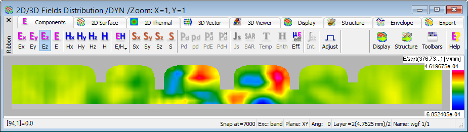
Fig. 2.5.2-5 Vertical electric field at 7000 iteration of wgf analysis – 2D Thermal display: simplified Discrete (upper) and Continuous (lower) with Shape and Isotropic options.

Pressing  button for the second time invokes 2D/3D Fields Distribution window in 2D Thermal Discrete display as shown in the upper part of Fig. 2.5.2-5. We may switch to 2D Thermal Continuous display by pressing  button in 2D Thermal tab of 2D/3D Fields Distribution window and we obtain the lower display of Fig. 2.5.2-5.

In any thermal display, placing the cursor over a particular cell in the 2D/3D Fields Distribution window brings the field value in this cell into window status bar. We can see that the field has decayed to the level of 10^-4, and thus we expect that the simulated results have converged. We press  button in S-Parameters section of Results tab of QW-Simulator to invoke the Results window with S-Parameters results. We obtain the display of |S11| in linear scale as in Fig. 2.5.2-6.

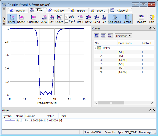
Fig. 2.5.2-6 Absolute value of reflection coefficient of wgf filter in linear scale.

QW-Simulator offers many ways of modifying the contents, scale, and layout of Results window . Their detailed discussion is given in Results Display. Here let us show how the most frequently used options can be activated.

The cursor is moved with left mouse button. Pressing N or P on the keyboard shows the next or previous calculated curve. To display several curves on one display we invoke Config dialogue and choose the curves to be displayed from the list of available characteristics. The Config dialogue allows also to calculate new characteristics based on the available ones. For example, if we highlight |S21| (by pressing left mouse button over it) and then press Show, we will see |S21| alongside with the previously shown |S11|.

Press  button for the second time. The Results window with |S11| and |S21| curves in linear scale will appear. We can change scale to decibel in Scale tab of Results window ( button). We can also change scale limits by pressing  button. This invokes Scaling dialogue, which with the contents shown in the middle of Fig. 2.5.2-7 produces the display shown at the top of Fig. 2.5.2-7.

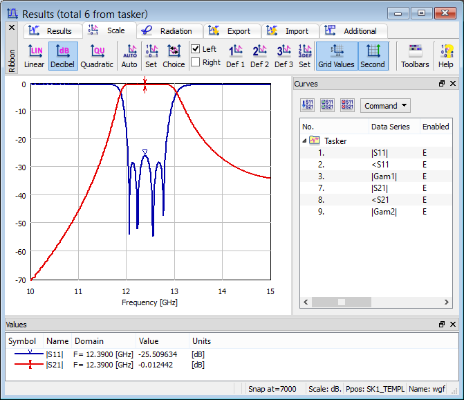
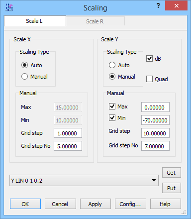
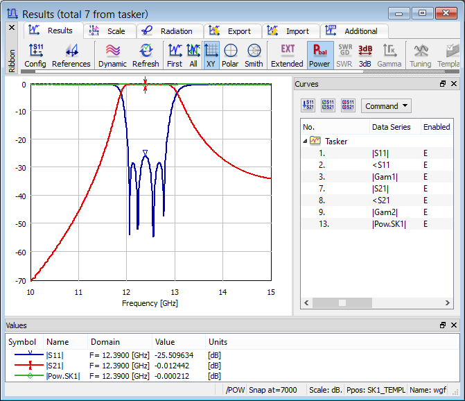
Fig. 2.5.2-7 Absolute values of reflection and transmission coefficients of wgf filter in decibel manual scale, and a Scaling dialogue applied to produce this display, and the S-parameters results with power balance curve.

Fig. 2.5.2-7 shows a pass-band (with nearly full transmission and reflections below –25 dB) in the centre of the considered frequency band. A question arises, if this is the final result, that is, if the FDTD process has converged. QW-Simulator allows verifying the convergence in several ways, of which the following ones are applicable here:

·       We may use energy simulation stop criterion feature. This feature allows suspending/stopping simulation, when energy accumulated in the circuit decays to user defined relative level (compared to maximum energy value). This is a very useful and convenient mechanism since it is fully automatic.

·       Since we are calculating S-parameters of a lossless multiport, we can check the balance between output and input power, which should approach unity. We invoke power balance curve by pressing  button in Results tab of Results window. We obtain the curve shown at the bottom of Fig. 2.5.2-7.

·       We note that all the curves are smooth. In a transient state, they would be corrupted with ripples. We will come back to this issue later.

·       We can also check that the calculated characteristics remain constant in time if we continue the simulation. We click  button to resume the simulation. We then refresh the Results window display either manually by pressing space bar on the keyboard, or dynamically by switching on the Dynamic mode ( button in Results tab of Results window or D on the keyboard). We find that changes of the |S11| and |S21| curves are below observable levels. Placing the cursor in the passband we note that the numerical value of |S11| fluctuates at the fourth decimal digit, at the -25 dB level. In the stopband, |S21| fluctuates at the second decimal digit, at the –70 dB level.

·       We can also look at the level of fields remaining in the filter. As we have already checked, they have decayed to the 10^-4 level. This confirms that power remaining in the filter is negligible, when compared with input power resulting from the source available power of 1W.

To repeat the above FDTD analysis process from the beginning, there is no need to come back to QW‑Editor. We can just press  button and then  button, both from Run tab of QW-Simualtor.

To make changes in the geometry, excitation, post-processing functions etc. we press  and exit QW-Simulator to get back in QW-Editor.

Modifying excitation:

A nice feature of the FDTD method is that we can dynamically watch wave propagation through the circuit. It is especially instructive in sinusoidal excitation regime.

Thus in QW-Editor please invoke Edit Transmission Line Port dialogue for source port pxin. On the Waveform list (Parameters tab) select sinusoidal and set Frequency f1: 12.39 GHz. Press OK and then  button from Simulation tab of QW-Editor.

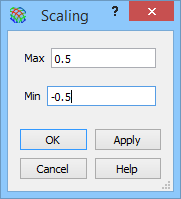
Fig. 2.5.2-8 Scaling dialogue for 2D Thermal field displays. Its units for electric field are [V/mm]*sqrt(120p), for magnetic fields  [A/mm]/sqrt(120p).

QW-Simulator reaches the steady-state after about 2000 iterations. After invoking second 2D/3D Fields Distribution window (by pressing  button in 2D/3D Fields tab) we obtain a field display governed by the last settings of the previous run of the same project showing Ez component of electric field, as previously, and apply a Continuous mode ( button in 2D Thermal tab ). To fix the scale of the display, please invoke Manual option under  button in 2D Thermal tab, and set the Scaling dialogue as in Fig. 2.5.2-8. The principles of field normalisation in QW-3D are explained in Electromagnetic fields; here let us only mention that 0.5 for electric field means 0.5* sqrt(120p) [V/mm].

This mode of display is very slow, but visualises in an intuitively appealing way the process of energy propagation through the filter. The snapshots of Fig. 2.5.2-9 have been taken at 7 iterations intervals. We can consult Simulation Info tab of Simulator Log window to see that the time step dt is equal 0.00169797 ns. Thus 0.02377 ns have elapsed between the uppermost and lowermost display, which is 30% of the period at 12.39 GHz.

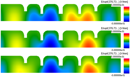
Fig. 2.5.2-9 Snapshots of instantaneous E_z field distribution in a 2D Thermal Continuous mode with Shape option on, in manual scale of [-0.5..0.5]*sqrt(120p) V/mm, at 7 iterations intervals.

In sinusoidal steady-state, field envelopes are even more meaningful that the instantaneous fields as they reveal the regions of inherently low and high energy concentration, and reproduce travelling or standing wave patterns. The plane envelope maximum of the currently monitored field component can be produced by pressing  button in Envelope tab of 2D/3D Fields Distribution window (or E on the keyboard). Remember that it only works in dynamic mode, indicated by /DYN in the window title bar. When envelope is switched on, the title bar shows by /DYN/Env Max . Constructing the envelope in 2D Thermal Continuous mode is possible but very slow. Thus it is advisable to switch to one of 2D Surface modes (in 2D Surface tab of the 2D/3D Fields Distribution window) and then back to 2D Thermal Continuous (in 2D Thermal tab of 2D/3D Fields Distribution window) when the envelope is stabilised.  Since the envelope values are by definition non-negative, we modify the scale to 0..0.5. At the considered pass-band frequency of 12.39 GHz we obtain the upper picture of Fig. 2.5.2-10.

We now press  button, exit QW-Simulator, back in QW-Editor invoke Edit Transmission Line Port for source port, and change Frequency f1: 11 GHz. Press OK and then  button. The steady-state envelope, in the same 0..0.5 scale, is shown in the lower part of Fig. 2.5.2-10. It confirms that we are in a stop-band, and the wave does not enter the consecutive resonators.

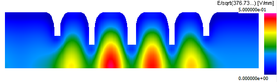
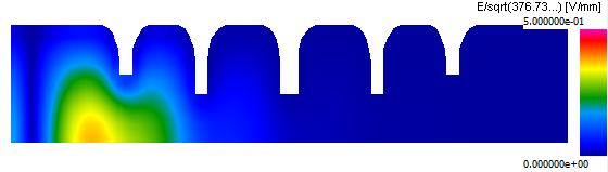
Fig. 2.5.2-10 Envelope maximum of E_z field distribution in a 2D Thermal Continuous mode with Shape option on, in manual scale from 0 to 0.5*sqrt(120p) V/mm: at 12.39 GHz (upper) and at 11 GHz (lower).

From field envelopes we should be able to extract the standing wave ratio (SWR), and hence to verify our earlier calculations of the reflection coefficient. However, in our wgf.pro example the input waveguide section is too short to accommodate at least one maximum and one minimum. We will try to prolong this section. To this end, we exit QW-Simulator and come back to QW-Editor.

Modifying geometry:

As it has been stressed in previous examples, the most convenient way of modifying geometry is by updating the parameters of the utilised UDOs. Our wgf.pro has been created from a single filters\wgsfil.udo. We can investigate the parameters available for modification by Select Object  ( button in 2D Window of QW-Editor) and double-clicking over wgsfil.udo. We can see (Fig. 2.5.2-11) that the parameters include, among others, waveguide width and height; width and thickness of consecutive irises; length of consecutive resonators. Filter order as well as rounding radius for resonators are also available.

This choice of parameters indicates that wgsfil.udo has been designed for fast frequency-domain analysis and optimisation of waveguide filters of various orders (n=3-7), for various frequency ranges, with various characteristics. It has not been designed for tutorial purposes such as extracting SWR from time-domain field envelopes. In particular, we cannot see any immediate way of extending the input waveguide length.

We have several options. One is to modify wgsfil.udo and create our own script, with input waveguide length directly available in the header. This option would be advisable if we were going to perform many experiments modifying waveguide length. However, since we want to run just one validating simulation, we may find it easier to add a waveguide section to the wgf project but outside wgsfil object.

We can press , browse the libraries and call basic/solid.udo with parameters:  30,9.525,9.525,air,E,0 and origin -30,4.7625, 4.7625.

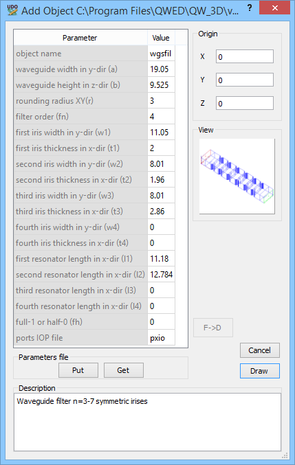
Fig. 2.5.2-11 Header of wgsfil.udo object.

Alternatively, we can add an element manually. We proceed as follows:

·       press ,

·       in the Define Level dialogue set Level Z 0, Default H 9.525, Medium air, Bottom/top kind Electric.

·       press  (which is a shortcut for drawing cuboidal elements),

·       press K for accurate keyboard entry of coordinates,

·       in Keyboard Entry dialogue set –30, 0,

·       press K again,

·       in Keyboard Entry dialogue set  0, 9.525.

Now the waveguide section is longer, but input port is placed inside it. To move the port to the edge we press ; double-click over pxin; make sure that the cursor is now square in the 2D Window of XY-plane; click right mouse button; in the Edit I/O Port dialogue set the box Shift X to –30 and press OK. New position of the source port can be also set in the Edit Transmission Line Port dialogue.

Now press . The steady-state envelope constructed as previously is shown in the upper part of Fig. 2.5.2-12. Moving the cursor over this display we read the maximum value of 0.341929  and minimum of 0.0114827, indicating SWR=29.8.

We can also make immediate SWR readings in 1D Fields window. We invoke it by pressing  button in 1D Fields tab of QW-Simulator. The dialogue is set to show Ez component of electric field along X axis (Domain: X) with Y and Z Position set to 3 and 2 respectively. The Markers has been activated ( button in Scale/Functions tab of 1D Fields window). Place the markers at the maximum and minimum of the envelope maximum curve and press  button (in Scale/Functions tab) to calculate the SWR value. The result is shown in the lower part of Fig. 2.5.2-12. The calculated value is SWR=27.8, which corresponds to calculated |S11|=0.9306, and is close to that deduced from the 2D envelope. Finally, let us note that the S-parameter extraction with pulse excitation has produced |S11|=1.000. The 1D Fields window readings produce lower values of |S11| because of limited mesh resolution in the X-direction, which causes that the actual envelope minimum is not found because it does not coincide with any of the E_z nodes. We can check that refining the mesh in the X-direction to 0.3 mm gives |S11|=0.97, and to 0.1 mm – |S11|=0.99.

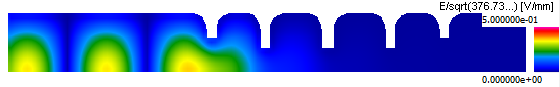
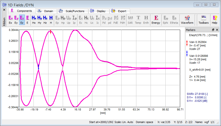
Fig. 2.5.2-12 The 2D (upper) and 1D (lower) envelopes of E_z at 11 GHz.

Modifying materials:

Let us return to QW-Editor and the original wgf.pro example. So far we have been dealing with an idealised lossless model. In practical realisations, metal losses may have an important influence on filter performance.

Open Project Media and the first medium on the list, available for editing, is metal, by default defined as PEC (perfect electric conductor). With the settings of Fig. 2.5.2-13, we assign to it surface losses governed by conductivity Sigma of 10⁵ S/m. Press  to save these settings, and then .

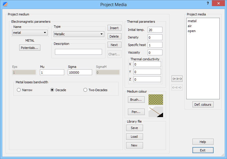
Fig. 2.5.2-13 Setting metal losses in wgf.pro.

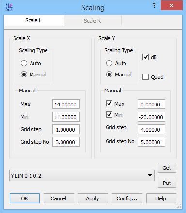
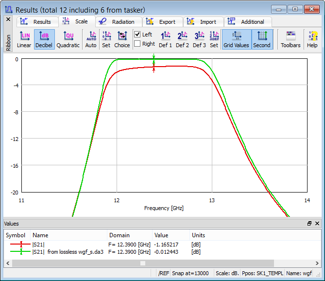
Fig. 2.5.2-14 Transmission through the lossless and lossy wgf filter.

Clicking  starts the simulation, and  displays the results. In Import tab of Results window we press  button and load wgf.da3 with the results of a lossless case which are included in the installation examples; then in Config dialogue, mark the two |S21| curves (positions 4 and 10 on the list), and press Show Sel. button; finally choose Decibel scale and invoke Scaling dialogue ( button), then make settings as on the left of Fig. 2.5.2-14. We obtain the display as on the right of Fig. 2.5.2‑14.

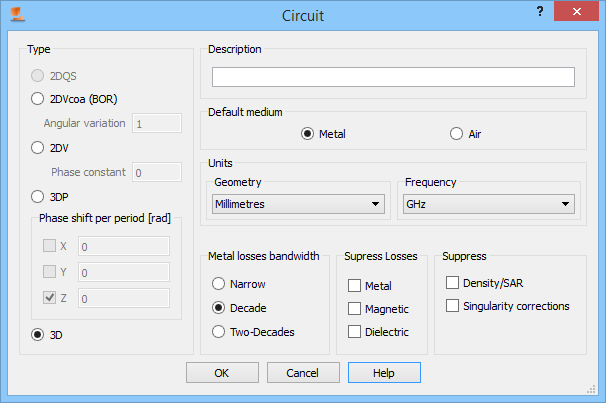
Fig. 2.5.2-15 Recommended Circuit setting for lossy wgf analysis.

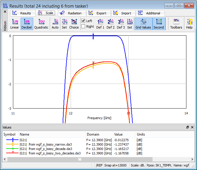
Fig. 2.5.2-16 Transmission through the lossless (blue) and lossy wgf filter – with skin effect accurately modelled over narrow band (yellow), decade (green) and two decades (red, overlaps green).

For details of metal loss modelling, please refer to Metallic. Here let us only note that the above analysis has been performed with the default model, which provides accurate results over one decade frequency range. QW-3D offers the choice of three models accessible via Project Media dialogue (Fig. 2.5.2-13) and Circuit dialogue of QW-Editor. In the Circuit dialogue of Fig. 2.5.2-15 we find the field Metal losses bandwidth with options Narrow, Decade, Two Decades. All these options rigorously model the skin effect in the centre of the considered frequency band, and approximate its frequency dependence by a ladder of LR elements. The ladder is shortest for Narrow option, causing that the simulation is fastest, but its accuracy visibly deteriorates with one frequency decade. The ladder is longest for Two Decades option, providing precise results within two decades bandwidth, but at the expense of prolonged computations. The default Decadeoption is a compromise between bandwidth and speed requirements.

Note that our wgf transmits the fields within a narrow (about 7%) frequency band, so we can actually apply a faster Narrow model without any loss of accuracy. Fig. 2.5.2-16 compares the results of the lossless filter with those of a lossy one, modelled with each of the three options.