2.3.2 NTF transform in open space and with infinite ground plane
In typical NTF transformation we use open space Green’s function. Thus we assume that:
· NTF surface surrounds entirely the considered radiating object,
· NTF surface is situated entirely in air,
· outside NTF surface we have only absorbing boundaries.
This is a situation well exemplified by the horn1.pro example presented in Fig. 2.3.1-1. To supplement the above conditions by practical remarks concerning their application in QW-3D let us note that:
· NTF surface can be relatively close to the radiating object. Two-three cells of separation are usually sufficient in the case of antennas fed by transmission lines. A bigger distance may be required in the case of dipoles radiating in free space since they can generate quasistatic mode around them and perturb the correct calculation of radiated power with “from NTF fields” option.
· The separation between NTF surface and absorbing boundary must not be smaller than three FDTD cells. Otherwise the far field calculation may be incorrect. Note that QW-Editor displays full cells in XY plane but half-cells in XZ or YZ planes. Thus when watching the QW-Editor displays in XZ or YZ we need to make sure that a distance of at least six half-cells is maintained.
The absorbing boundary can be placed quite close to the antenna providing that the antenna does not generate evanescent modes sliding along the boundary. In the latter case, from the physical viewpoint, an absorbing boundary should be neutral to the wave. However, in practical numerical solutions it may generate small amounts of energy and inject them back into antenna. This may deteriorate the accuracy of the analysis of high-Q resonant antennas and sometimes even lead to instability of the FDTD simulations. Such a possibility should be considered in the analysis of planar antennas and will be exemplified in Patch antenna. Here let us only note that a cure to this problem is placing the absorbing boundary at a bigger distance from antenna. The distance of half a wavelength is usually sufficient.
Fig. 2.3.2-1 QW-Editor display of the example horn2.pro.
QW-3D is able to provide correct far field patterns not only in open space, but also in the cases when the space is limited by one, two or three electric or magnetic planes perpendicular to X, Y or Z axes. This is accomplished by appropriate modification of Green’s function within the NTF transform. There are two practical applications of this feature:
· The first application concerns the situation, in which we want to assume infinite ground plane below the antenna. It is exemplified by horn2.pro later in this Section.
· The second application concerns symmetrical structures, in which the computational domain can be restricted to half, quarter or one-eighth of the entire domain. It is exemplified by projects with sets of dipoles in Manual operation of QW-Editor.
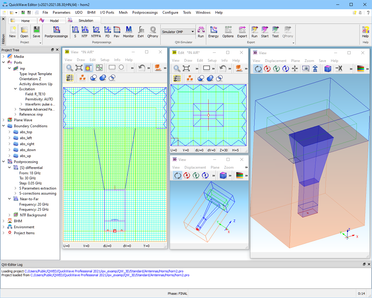
Let us now consider the example horn2.pro presented in Fig. 2.3.2-1. It concerns a rectangular waveguide horn of the same size as in example horn1.pro. However, this time the horn is placed inside a big block of metal and we shall assume that the block is infinite in the XY plane. In Fig. 2.3.2-1 we can see that the NTF box has been situated entirely above the metal block. Moreover, the absorbing box contains only 5 absorbing walls – no absorbing wall is needed below the block.
Actually, in each of the examples: horn1.pro and horn2.pro the combination of the NTF and absorbing boxes has been drawn using ntf.udo, which can be found in the library boxes. Fig. 2.3.2-2 shows the header of this UDO with parameters set in either case. Besides the dimensions of the NTF and absorbing boxes, there are three parameters concerning possible introduction of particular symmetry conditions at infinite planes situated in X=0, Y=0 or Z=0. In each of the planes we may have N – no specific conditions, E – electric-wall symmetry conditions, or M – magnetic-wall symmetry conditions.
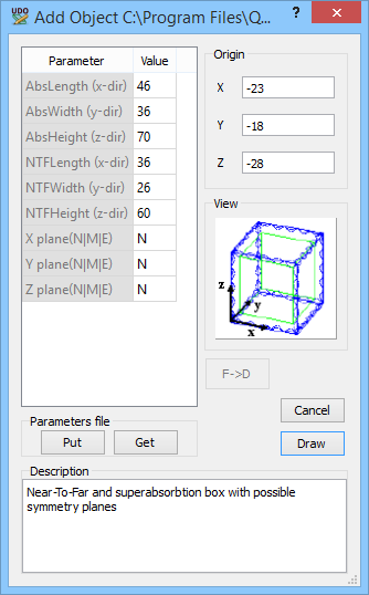

Fig. 2.3.2-2 Header of ntf.udo with parameters used in horn1.pro (left) and horn2.pro (right).
In the case of horn1.pro no special conditions have been declared. In such a case the NTF box must surround the entire structure and the software will calculate the NTF transformation from a free-space Green’s function. In the case of horn2.pro we have declared the electric symmetry plane for Z=0. The software will calculate NTF transformation using a Green’s function applicable to this case. Note that the above declarations of symmetry planes concern the method of NTF calculations, and not the geometry of the project. In other words, the software does not enforce a metal plate all over the XY-plane at Z=0 horn2.pro. This allows the horn to radiate through its aperture. However, it is the user’s responsibility to assure the consistent electric-wall boundary conditions over this plane except for the aperture. In horn2.pro this is provided by locating the NTF box directly upon the metal block, which spans the full XY-plane between the edges of the FDTD computational domain, up to the absorbing boundaries.
Radiation patterns produced by horn1.pro and horn2.pro for the Ephi polarisation is presented in Fig. 2.3.2-3. The green curve shows the results of horn1.pro (the same as presented in Fig. 2.3.1-6), while the blue curve shows the results of horn2.pro where an infinite ground plane has been assumed.
Note that a symmetry plane in the NTF transformation may model two physically different scenarios: radiation from a single source over a physical ground plane (which is the case in horn2) or a symmetry plane in the system with two sources, reducing the simulation to a half-space (this is considered in Two dipoles in free space excited out of phase). Both case produce the same shape of the radiation patterns but with levels differing by 3dB. The user resolves this ambiguity by setting the actual Number of ground planes in the Radiation Patterns dialogue. The default is 0, corresponding to the two sources case; for horn2, the default is modified to 1 as in Fig. 2.3.2-3).
Compare the radiation patterns of horn1.pro and horn2.pro. The differences are very small in the main lobe from 0 to 600. At 900 the blue curve drops to 0 (-¥ in dB scale) because the considered polarisation cannot propagate along the metal surface (top of the metal block). In horn2.pro we assumed that we consider radiation in the half-space above the plane Z=0 and thus for Theta £ 900. The radiation pattern calculated above 900 is a mirror reflection of the pattern calculated below 900 and should be disregarded.
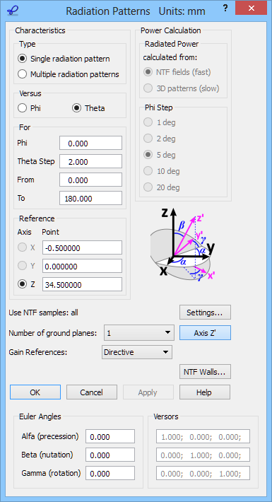

Fig. 2.3.2-3 Comparison of radiation patterns calculated with horn1.pro (green) and horn2.pro (blue). The upper picture shows the Radiation Patterns settings used for horn2.
We may also look at the Poynting vector at both NTF frequencies, namely 20 and 25 GHz, incorporating Frequency Domain Monitors (more details in Joint use of contours with frequency-domain monitoring of fields and source signal). Consider horn1_fdm.pro example where FD Monitors have been set in XZ and YZ cross-sections of the horn at 20 and 25 GHz. Fig. 2.3.2-4 and Fig. 2.3.2-5 show the real part of the complex Poynting vector in YZ plane obtained at the two frequencies, respectively. The windows are invoked by pressing Monitor button (![]() ) from Monitor tab of QW-Simulator two times.
) from Monitor tab of QW-Simulator two times.
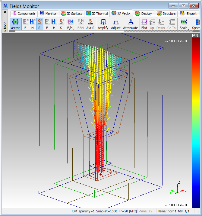
Fig. 2.3.2-4 Real part of the complex Poynting vector in YZ plane at f = 20 GHz (horn1_fdm.pro).
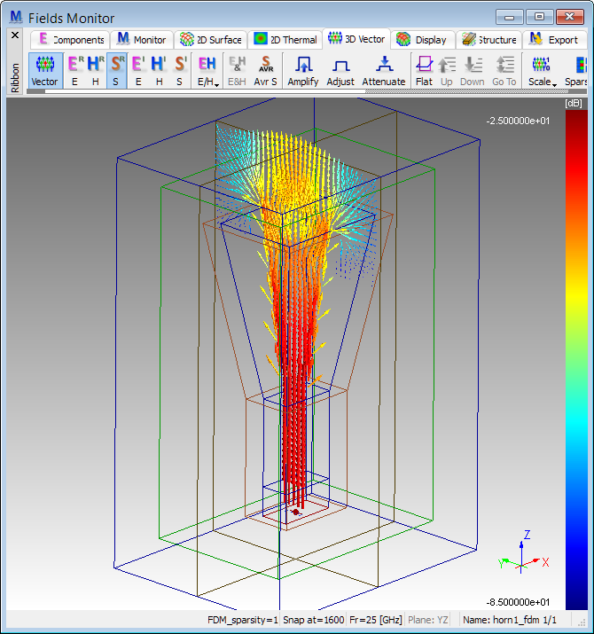
Fig. 2.3.2-5 Real part of the complex Poynting vector in YZ plane at f = 25 GHz (horn1_fdm.pro).
Attention: FD Monitors described in this Section are two-dimensional. They provide information about distribution of the fields on a two-dimensional flat frame. They can be introduced into our project using UDOs available in QW-library (named: fdmx.udo, fdmy.udo and fdmz.udo). Since version2012 a new approach to the FD Monitors is available. UDO named fdm3d.udo defines 3D box for field monitoring. That kind of approach is much more flexible than the previous one and provide better possibilities of field monitoring. Thus they are recommended for all new projects. Example of application of the FD Monitors 3D is shown in Application of Frequency Domain Monitors (FDM) for microwave heating. It is still possible to use the old 2D monitors but that option is kept mostly for compatibility with older projects.
Since version 2012, FD monitors can be computed in a specified volume (more details see in Application of Frequency Domain Monitors (FDM) for microwave heating). Consider horn1_fdm3d.pro example where FD Monitor 3D has been set at 20 and 25 GHz with FDM spatial sparsity equal 2. Fig. 2.3.2-6 shows the real part of the complex Poynting vector at f = 20 GHz. The window is invoked using Monitor button (![]() ) from Monitor tab of QW-Simulator. Please note that because of the FDM spatial sparsity is greater than 1, the results of Poynting vector are estimated.
) from Monitor tab of QW-Simulator. Please note that because of the FDM spatial sparsity is greater than 1, the results of Poynting vector are estimated.
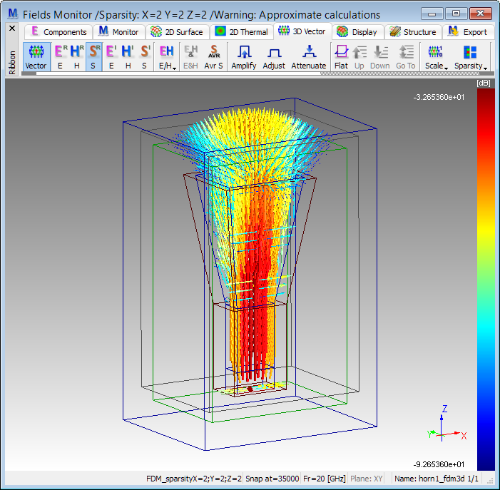
Fig. 2.3.2-6 Real part of the complex Poynting vector at f = 20 GHz (horn1_fdm3d.pro).