2.19.1 Shape optimisation using Matlab - rwgconv example
QW-OptimizerPlus available as a part of the QuickWave package is a useful and easy-to-use tool in optimisation projects where the goal is to optimise S-parameters or radiation pattern of a microwave structure by adjusting specified parameters of that circuit. However, when it comes to more complicated tasks like optimisation of a complex shape of some structure, Matlab and other computational environments may have an advantage over closed, highly-specialised tools like QW‑OptimizerPlus.
Consider a rectangular waveguide mode converter as an example of such complex project. All files used in this example require that the user has an access to Matlab version 6.0 or newer. A mode converter is a lossless microwave structure in which the wave at the input propagates as the m-th mode but it reaches the output as the n-th mode, and the m ¹ n. It is also important to ensure that mode conversion is done efficiently or that the energy of the output mode is as close as possible to the energy of the input mode.
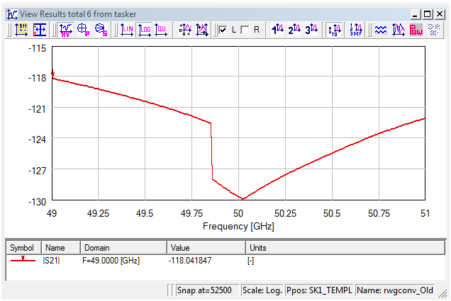
Fig. 2.19.1-1 illustrates the S21 curve of a microwave circuit consisting of a straight piece of a rectangular waveguide of cross-section 10.0´5.0 mm used as a mode-converter. The input mode is TE10 while TE30 has been chosen as the output mode. In this geometry the cut-off frequency of the input and output mode is 15 GHz and 45 GHz, respectively. The working frequency should be higher that the output mode cut-off so we can safely choose 50 GHz. The input port of the waveguide can be configured by selecting the R_TE10 mode from the drop-down list in the Add Transmission Line Port /Edit Transmission Line Port dialogue, while the output port should be configured by selecting Arbitrary from the list and typing 0.19 in the Effective permitivitty box. Because these two modes are orthogonal the efficiency of the conversion is zero, and it is obvious that a more complicated solution to the formulated problem is needed.
Fig. 2.19.1-1 Efficiency of a straight piece of waveguide used as a mode-converter.
In order to make the conversion one can purposefully deform one wall of the waveguide in order to generate the TE30 mode missing at the input. If the deformation process is closely controlled one can expect to obtain a better result.
The shape of the waveguide wall can be easily controlled with just a few points. If some interpolation algorithm is employed then based on the position of those points the entire shape can be described. In such an approach only limited number of parameters is needed by an optimisation algorithm to modify the shape of the waveguide wall while increasing the efficiency of the conversion.
The selected interpolation algorithm should ensure smoothness of the wall in order to avoid introducing singularities inside the waveguide. A numerical method which seems to be a good candidate is splines-based interpolation. In Matlab environment one can use a ready-made routine spline that implements this method. Fig. 2.19.1-2 presents three example curves obtained for three sets of control points. The legend shows only the y-position of each control points – they are equispaced along x-axis. The control points are marked with circles.
Using the spline interpolation algorithm it is possible to design the shape of the waveguide wall in the Matlab environment based on a few parameters and transfer it to a QuickWave project through a text file. After its creation, the file can be opened by a UDO object which can draw a piece of the rectangular waveguide according to the shape description prepared by Matlab. If the UDO can additionally prepare ports, then one has a full project that can be modelled by the QW-Simulator.
All those steps are realized by the getShape.m and qw.m Matlab scripts and the rwgconv.udo object that can be found in the rwgconv folder. The first script accepts the specified number of control points and uses them to constructs the wall shape. Then the qw.m script is called which saves the shape data to a text file, calls the QW-Editor to prepare the modified project with the new shape. Finally the QW‑Simulator is called to obtain new S21 parameters. The S21 curve is returned by the getShape.m script. The S-parameter analysis is performed in the frequency band of 49 GHz to 51 GHz. The getShape.m script further narrows the band because the designed mode converter is to work for the frequency of 50 GHz and taking into account more frequencies would make the optimisation process unnecessarily complicated.
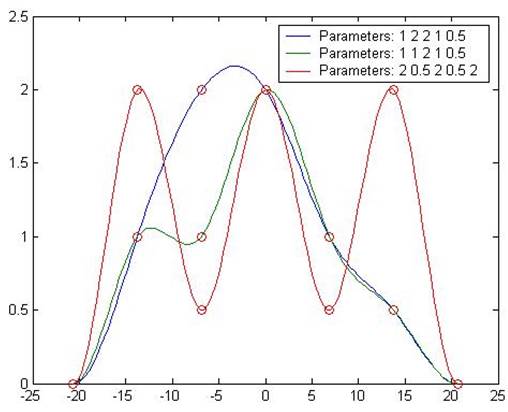
Fig. 2.19.1-2 Three example curves obtained with spline interpolation algorithm.
The rwgconv.udo draws the whole QuickWave project together with the input and output ports and the initial and final section of the circuit. The shape of the middle section of the waveguide is read directly from the text file prepared previously be the getShape.m Matlab script.
Now, that everything is ready one can start the optimisation. As the starting point for the search a bell curve is proposed. In order to make the optimisation run smoother and to limit the number of optimised parameters only the y-positions of the control points will be changed. An assumption is made that the x-positions of the control-points will stay fixed and that the gap between the points is equal to the half of the wavelength of 50 GHz mode TE30 wave.
In order to further simplify the process, the positions of the control-points are not passed to the getShape.m script directly. With the exception for the first parameter they are defined in relation to the previous parameter. For example, if 5 control-points is used with the following y-positions: 1.0, 2.0, 3.0, 2.0, and 1.0, the getShape.m script should receive the following sequence: 1.0, 1.0, 1.0, 1.0, 1.0. The first parameter is simply the position of the first control-point. The value of the 2nd parameter has been obtained by subtracting positions of the 2nd and 1st control-points. The value of the 3rd parameter comes from subtracting positions of the 3rd and the 2nd points. The same approach has been employed for the rest of the parameters but with the assumption that their value is smaller than the value of the 3rd parameter the result of the subtraction is multiplied by –1.0.
The getShape.m script will rebuild the y-positions of the control point based on the received data, calculate the shape of the wall and with the help of the qw.m script will perform the simulation of the structure.
Fig. 2.19.1-3 illustrates the result obtained for the starting shape – the bell curve drawn with 5 control-points whose y-positions are given as: 2.0, 10.0, 16.0, 10.0, and 2.0 mm (which results in the following sequence passed to the getShape.m script: 2.0, 8.0, 6.0, 6.0, 8.0). As can be seen the conversion is far from perfect and some work needs to be done on improving the efficiency of the conversion. Also a look at the S21 curve reveals that there is still lots to do – the value of 0.3 is obviously not enough.
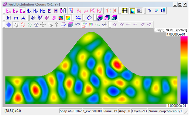
Fig. 2.19.1-3 The Ez field in the mode converter structure – the starting shape.
The optimisation process can be run from another script – conv.m script. Inside there are definitions of the paths leading to the QW-Editor, the QW-Simulator and the project files as well as the number of control points, some parameters of the optimisation routine and the call to the optimizer itself. It should be noticed that the user needs to adjust the paths in conv.m script according to the local settings. As can be seen, the fminimax function is used. It sequentially calls getShape.m script with various sets of the parameters. Fig. 2.19.1-4 illustrates the contents of the Matlab script after the routine has converged to a solution.
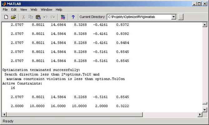
Fig. 2.19.1-4 The result of the optimisation process – 85% compared to the initial 32% conversion efficiency.
The field distribution inside the optimised structure has been presented in Fig. 2.19.1-5. The cleared TE30 at the output is clearly visible. The improvement of the efficiency can be attributed to the dent that formed in the waveguide wall close to the output. The structure inside the QW-Editor is presented in Fig. 2.19.1-6.
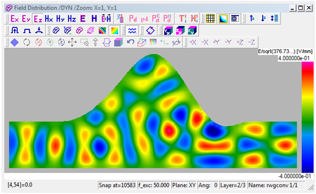
Fig. 2.19.1-5 The Ez field in the mode converter structure – the optimised shape.
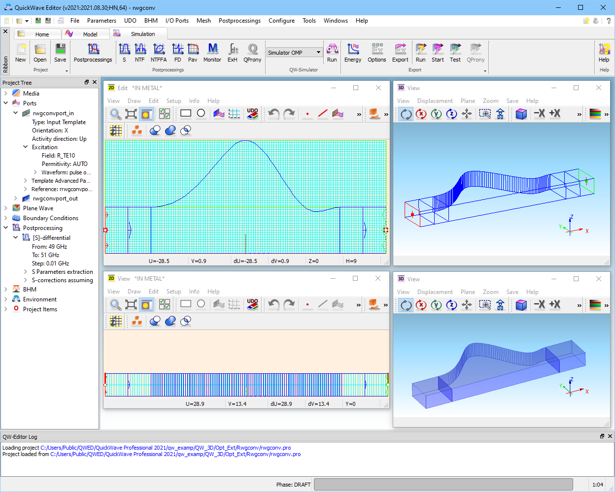
Fig. 2.19.1-6 The optimised shape of the mode converter in the QW-Editor.
The comparison of the S21 curves obtained for the initial shape and the optimised project has been shown in Fig. 2.19.1-7. In order not to make the optimisation process too complex the reflection coefficient has not been taken into account which resulted in high reflections reaching 0.21 value in the optimised case. After a small modification of the optimisation script also S11 curve could be used be the fminimax function which would give much better efficiency. Also increasing the number of the control-points, or adjusting their x-positions would bring further improvement.
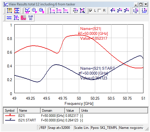
Fig. 2.19.1-7 Comparison of the S21 curves of the starting case (blue) and optimised case (red).