2.17.4 Specular scatterometry
In Plane wave excitation a versatile method for the analysis of plane wave illumination of periodic structures has been introduced. This method is applicable not only for the specular (0th order) scatterometry but also for the evaluation of higher order modes. However, sometimes we know a priori that higher diffraction orders will not appear in the scenario and we expect only the specular reflection. In such a case, we may take the advantage of a robust technique already introduced in Waveguide-to-coax transition, namely waveguide template source with S-Parameters extraction.
We may justify its applicability for the specular scatterometry in the following way. Each waveguide mode may be understood as a ray that propagates along the waveguide reflecting from the lateral walls at the particular angle of incidence αinc:
![]()
( 2.17.4-1)
where βz stands for the phase constant along the waveguide, β0 is a free space phase constant and αinc is inclined from the longitudinal waveguide axis.
We obtain a standing wave distribution in the waveguide cross-section. We may take the advantage of this phenomenon for the plane wave illumination in a periodic scenario provided that higher diffraction orders will not appear. Otherwise, the results would be disturbed.
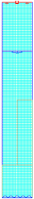
Fig. 2.17.4-1 Mesh view of grating_3dp.pro.
Open ...Scattering\Periodic\grating_3dp.pro example. The structure is composed of one period (Lx = 10 mm) of dielectric grating (εr = 2.2) with PBC applied along x axis (see Fig. 2.17.4-1). We assume that the substrate is of infinite depth so it may be truncated with the absorbing boundary at the bottom. We illuminate the grating with TE polarized plane wave at αinc = 300 to extract the reflection coefficient at f = 15 GHz. It corresponds to (φ, θ) = (-600, 900) in spherical coordinates. We need to synchronise the phase shift of the expected plane wave along one period of the grating with the Floquet phase shift per period ψx according to the eq. (2.17.1-1). In this case we get ψx = π/2.
According to eq. (2.17.1-2), we may check that higher diffraction orders do not propagate in this case so they will not disturb the |S11| calculation.

Fig. 2.17.4-2 Edit Transmission Line Port dialogue of grating_3dp.pro.
Invoke Edit Trasmission Line Port dialogue (see Fig. 2.17.4-2). Since we have chosen αinc = 300, according to the eq. (2.17.4-1) effective permittivity of the excited mode has to be set to εeff0 = 0.75. The same has been done with Mur absorption producing εeff1 = εeff0 εr = 1.65. We notice that the field will be excited around the frequency of our interest, i.e. from 13 up to 17 GHz.
According to eq. (2.17.1-1) the angle of incidence (AOI) is frequency dependent. In other words, pulse excitation produces a number of plane waves with AOI slightly varying with frequency. However, if a relatively narrow bandwidth is set we may assume that deviation of AOI may be neglected.
Fig. 2.17.4-3 shows the |S11| plot within the excitation band. We may notice that |S11| = 0.097741 at f = 15 GHz what may be understood as a reflection coefficient at 0th order. To verify this value we will analyse the same scenario but with the plane wave wall excitation and NTF transform (compare Plane wave excitation).
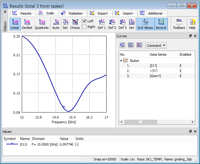
Fig. 2.17.4-3 |S11| of grating_3dp.pro.
Open grating_3dp_plw.pro. Comparing to the previous example, template source has been changed to the PLW wall, whereas NTF will serve to extract the reflection coefficient. After simulation run we obtain the scattering pattern shown in Fig. 2.17.4-4.
As mentioned in Plane wave excitation, vertical dashed lines indicate illumination and reflection angles. The reflection coefficient amounts to Rss = E(600)/E(3000) = 0.09708. Discrepancy is less than 1% as compared to |S11|.
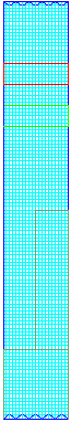
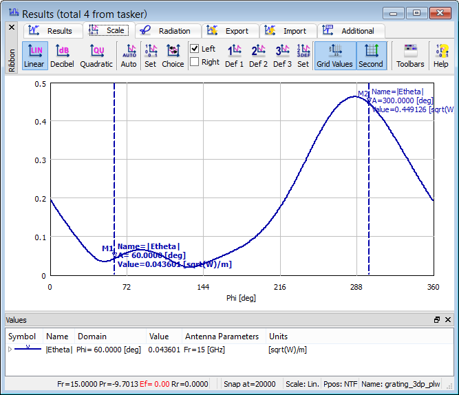
Fig. 2.17.4-4 Scenario considered in grating_3dp_plw.pro and its scattering pattern.
The Results window in Fig. 2.17.4-4 shows the radiated power Pr=-9.7013 [W]. Radiated power is defined as power outgoing through the NTF box. In this scenario, incident wave is injected by one plane wave wall (see Walls activity settings in Plane Wave dialogue of QW-Editor; uppermost red line in Fig. 2.17.4-4), and the flux is integrated through one NTF wall (see Pickup Walls settings via Radiation Patterns dialogue of QW-Simulator; uppermost green line in Fig. 2.17.4-4). The flux is incoming on this wall, and therefore the result of integration is negative.