2.15.2 Optimisation of a waveguide horn
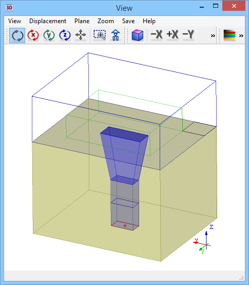
We consider the example Opt_Plus\Horn3\horn3.pro. It concerns a flat waveguide horn excited by the dominant waveguide mode (Fig. 2.15.2-1). An air-filled horn is assumed to be radiating from a block of metal (shown grey, semi-transparent). File horn3.udo is placed in the same directory. It describes the shape of the horn as well as the absorbing boundary above the metal block and the NTF box placed above metal with one E-type symmetry plane at the metal surface. In the optimisation process, we will be changing the horn length (in vertical z-direction) as well as its width (in x‑direction) and height (in y-direction). We will try to achieve good antenna gain for the frequency 24 GHz in the lobe of 0± 18° (in zx-plane) as well as good matching with |S11|<0.08 in the frequency range from 23.5 to 24.5 GHz.
Fig. 2.15.2-1 QW-Editor view of horn3.pro structure.
We proceed as in the previous example. We run the simulation to find that the results stabilise after about 1000 FDTD iterations. Then we stop the simulation and press ![]() button in Optimiser tab of QW-Simulator to set the optimisation parameters. We enable the hw, hh and hl variables. With respect to objectives, we concentrate here on two aspects which have not been considered before:
button in Optimiser tab of QW-Simulator to set the optimisation parameters. We enable the hw, hh and hl variables. With respect to objectives, we concentrate here on two aspects which have not been considered before:
- setting an objective based on antenna pattern calculations
- setting the goal function with two objectives.
After accessing the Objectives tab we can see that two different objectives are defined. Consider the second one. It indicates that we want to achieve the antenna directive gain of the Ephi polarisation with the target of 4.25 and lower bound of 2.83 in the sub-range of angles between 0 and 18 degrees. The range of the radiation pattern calculation will be broader, between 0 and 90 degrees, to give the user a picture of the pattern behaviour also beyond the sub-range of major interest. The pattern will be calculated with step 1 degree, and every point within the sub-range will be considered in the objective calculations (as seen by pressing the Sub-Range button).
After pressing ![]() and
and ![]() we obtain the dialogue of Fig. 2.15.2-2. It says that the radiation patterns will be calculated with respect to the Z-axis with angle phi set to 0 (i.e., in the ZX-plane). Actually, the range for angle theta has been set via this Radiation Patterns dialogue (and only copied to the Freq/Angle Range fields of the Edit Objective Linear Scale dialogue and into the Freq/Angle Lower and Freq/Angle Upper columns of the Objectives tab).
we obtain the dialogue of Fig. 2.15.2-2. It says that the radiation patterns will be calculated with respect to the Z-axis with angle phi set to 0 (i.e., in the ZX-plane). Actually, the range for angle theta has been set via this Radiation Patterns dialogue (and only copied to the Freq/Angle Range fields of the Edit Objective Linear Scale dialogue and into the Freq/Angle Lower and Freq/Angle Upper columns of the Objectives tab).
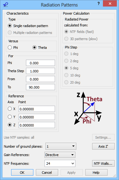
Fig. 2.15.2-2 Radiation Patterns dialogue used to define objectives in horn3.pro.
The radiation pattern objective will be calculated as:
GA= Max( 2.83- |Ephi(phi)| ) / (4.25-2.83) = (2.83 - Min( |Ephi(phi)| )) / 1.42
where the maximum / minimum is sought in the sub-range of theta between 0 and 18 degrees, with a step of 1°.
The first objective in the Objectives tab is based on the reflection coefficient in the Sub-Range between 23.5 and 24.5 GHz. This objective will produce:
GS = Max( (|S11(f)|-0.08) / (0.08-0)
where the maximum is sought in the sub-range of frequency between 23.5 and 24.5 GHz, with a step of 0.1 GHz.
QW-OptimiserPlus will take as its goal function the higher of the two values GA and GS.
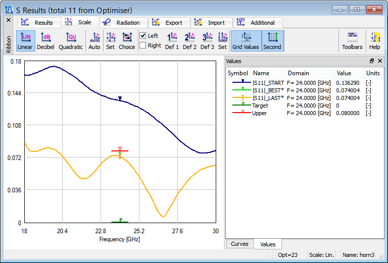
Fig. 2.15.2-3 Results of optimisation of the |S11| objective of horn3 example.
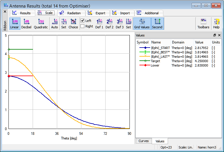
Fig. 2.15.2-4 Results of optimisation of the radiation pattern objective.
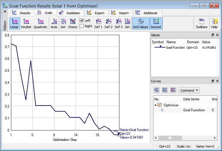
Fig. 2.15.2-5 Goal function progress during optimisation of horn3 example.
Start the optimisation with ![]() button. After 23 simulations QW-OptimiserPlus stops with the message: Target objective function value reached. We can see in Fig. 2.15.2-3 and Fig. 2.15.2-4 that both objectives have been fulfilled. Fig. 2.15.2-5 presents the progress of Goal Function, which drops below zero for simulation number 23.
button. After 23 simulations QW-OptimiserPlus stops with the message: Target objective function value reached. We can see in Fig. 2.15.2-3 and Fig. 2.15.2-4 that both objectives have been fulfilled. Fig. 2.15.2-5 presents the progress of Goal Function, which drops below zero for simulation number 23.