2.10.2    Basic example of application of SAT Filter

The  button in Model tab and Tools->SAT Filter command from main menu invoke SAT Filter Source and Options dialogue (Fig. 2.10.2-1) that allows setting the *.sat file and conversion parameters.

Let us consider an example stored as project ..\Antennas\Holen\holen1.pro. This project is ready to run. However, here we will assume that it is being built from scratch, based on the available ..\SAT\Holen\holen.sat file. SAT format is one of the most popular industrial formats, and many CAD packages use it as an optional output format. Note that, to be imported into QW-Editor, the *.sat file must be prepared according to compatibility rules with 3D volumetric modelling. The holen.sat has been prepared with a Modeller by Cobham Technical Services, Vector Fields Software and describes an antenna with lens geometry.

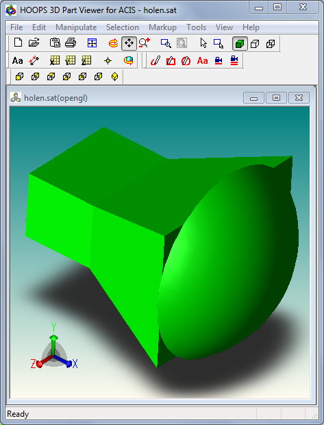
Fig. 2.10.2-1 View of holen.sat file in the free HOOPS 3D Viewer.

We will now make a SAT to UDO conversion step by step having a *.sat file, which contains two separate bodies, made of different media: the metal horn and the dielectric lens. SAT Filter module allows a conversion, where the medium of each cell contained in the sat file is a UDO parameter. In the conversion we will use holen.sat file. At the end we will compare the simulation result for the antenna obtained by the SAT to UDO conversion with the same antenna available in QW-3D examples (holen1.pro).

Having the QW-Editor opened, we load the project ...\SAT\Holen\holen.pro. Now invoke Tools->SAT Filter from main menu or  button from Model tab of the QW-Editor, and the SAT Filter Source and Options dialogue will appear (see Fig. 2.10.2-2). We Browse the  ...\SAT\Holen\holen.sat file. Under the Advanced button many useful, conversion options (described below) can be found.

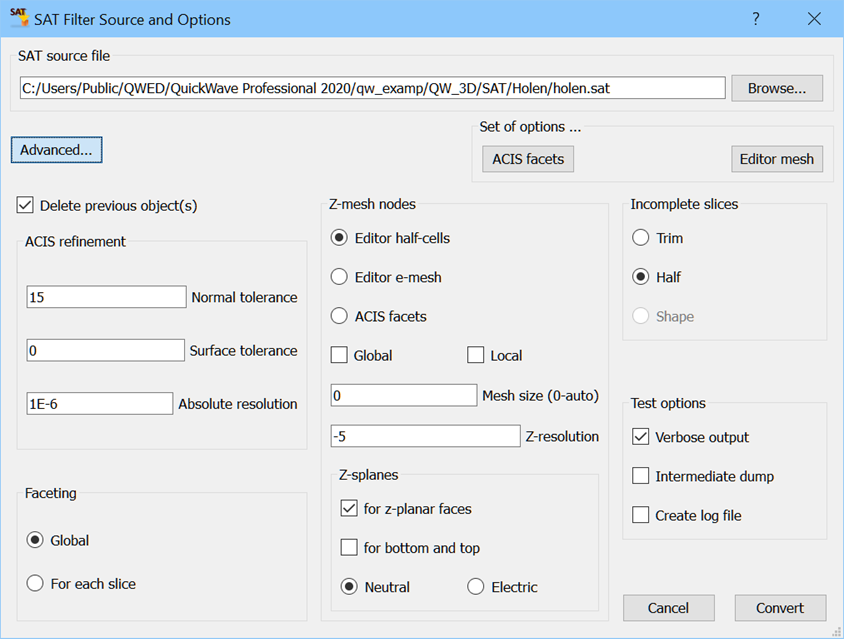
Fig. 2.10.2-2 SAT Filer Source and Options dialogue in typical form (upper) and in advanced mode (lower).

If the *.sat file have been chosen we can now make the first part of conversion, which can be called “creating the mesh”. We start this part by setting, in the Advanced window, Z-resolution equal to -1. Then we choose ACIS facets and press Convert.

We can say that, this stage generates only the size of the meshed area and this is the reason for which, most probably, the geometry will not look as we wanted. It is shown in Fig. 2.10.2-3, where the antenna after ACIS facets stage is presented.

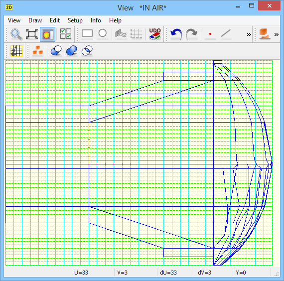
Fig. 2.10.2-3. The antenna object after ACIS facets stage of SAT to UDO conversion.

The second step in this part is defining mesh boundaries in the Mesh Parameters dialogue (Fig. 2.10.2-4). We press button Limits to XYZ and the size of the structure, from the first reading of *.sat file appears in Mesh boundaries (Adjust to Object checked). The size of the structure is defined by its minimum and maximum coordinate in a specific direction. In this case the dimensions in Z direction read from the *.sat file are not proper so we have to change them in a way shown in Fig. 2.10.2-4. If the dimensions of the structure placed in the mesh boundaries differ from its real dimensions, we should uncheck Adjust to Object and change the min, max values. In this step we have to generate the mesh with a proper cell size. It is especially very important in geometries like this one, where the curvatures appear. If the Max cell size is set to be 1 in all directions (like in holen1.pro) the geometry of the lens in Z direction is modelled not accurately enough.To get the accurate model of the lens we set the cell size equal to 0.5 in X and Y directions, 0.3 in Z direction (for comparison of the simulation results we will have to set the same cell size in holen1.pro) and we press Apply. If the precise dimensions of the structure are known, we do not have to make ACIS facets stage and we can simply define mesh boundaries in the first stage.

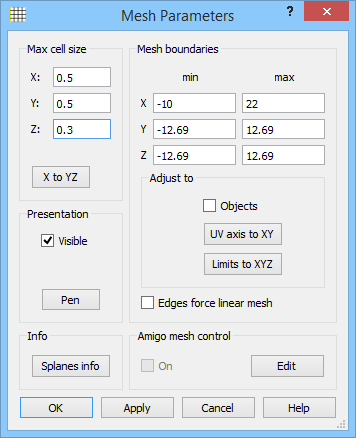
Fig. 2.10.2-4 Mesh Parameters dialogue window.

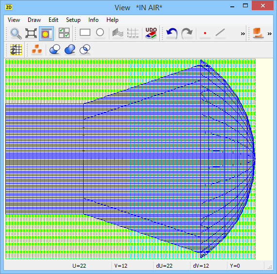
Fig. 2.10.2-5 The antenna object after SAT to UDO conversion.

When the mesh is prepared we can now go to the second part of the conversion which can be called “getting the structure”. In this stage once again we invoke SAT Filter Source and Options dialogue, but this time we press Editor mesh. This produces the antenna geometry, what is shown in Fig. 2.10.2-5.

The default setting is that all the converted body cells are air filled. Let us now change the medium settings for the horn and lens. In 2D Window we invoke Select Object dialogue ( button) and we choose holen object by clicking twice on the name. The window shown in Fig. 2.10.2-6 appears. Parameter Cell1_med which corresponds to horn medium should be changed to metal, and the Cell2_med to teflon.

After introducing these modifications we get the antenna shown in Fig. 2.10.2-7.

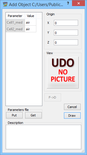
Fig.UG 2.10.2-6 The Add Object dialogue.

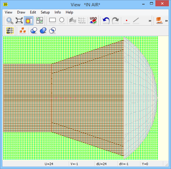
Fig. 2.10.2-7 The antenna object after media modifications.

To run the simulation and calculate the radiation pattern we have to introduce the NTF box and the exciting port in the project. We use the library objects boxes/ntf.udo and ports/portox.udo. To open objects library press  button in 2D Window. In Fig. 2.10.2-8 and Fig. 2.10.2-9, NTF and port geometry parameters can be found. The meshed area has to be now enlarged to include the NTF box. In Mesh Parameters dialogue, Adjust to Object option should be checked. In Edit Transmission Line Port dialogue we should set the port parameters as in Fig. 2.10.2-10. In Processing/Postprocesing dialogue we should activate S-Parameters and Near To Far post-processings, as shown in Fig. 2.10.2-11. We Save the project and run the simulation. In Fig. 2.10.2-12 and Fig. 2.10.2-13 the comparison of the simulation results (obtained with  and  buttons from Results tab of QW-Simulator), for the antenna obtained in the SAT conversion and the original one (holen1.pro with the Max cell size parameters set as in Fig. 2.10.2-4), can be found. Results are in very good agreement.

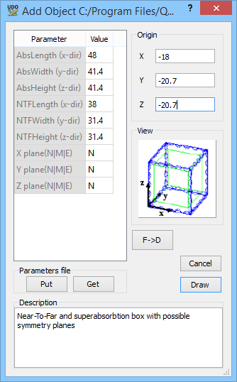
Fig. 2.10.2-8 Add Object dialogue for the NTF box.

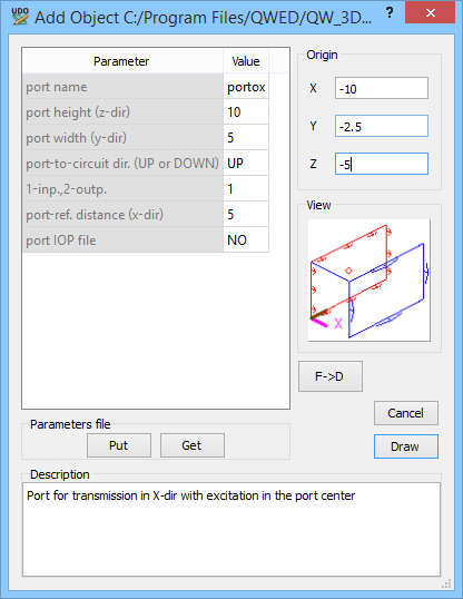
Fig. 2.10.2-9 Add Object dialogue for the port.

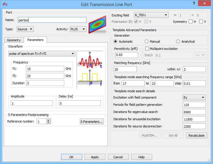
Fig. 2.10.2-10 Edit Transmission Line Port dialogue.

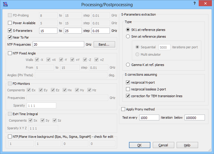
Fig. 2.10.2-11 Processing/Postprocessing dialogue.

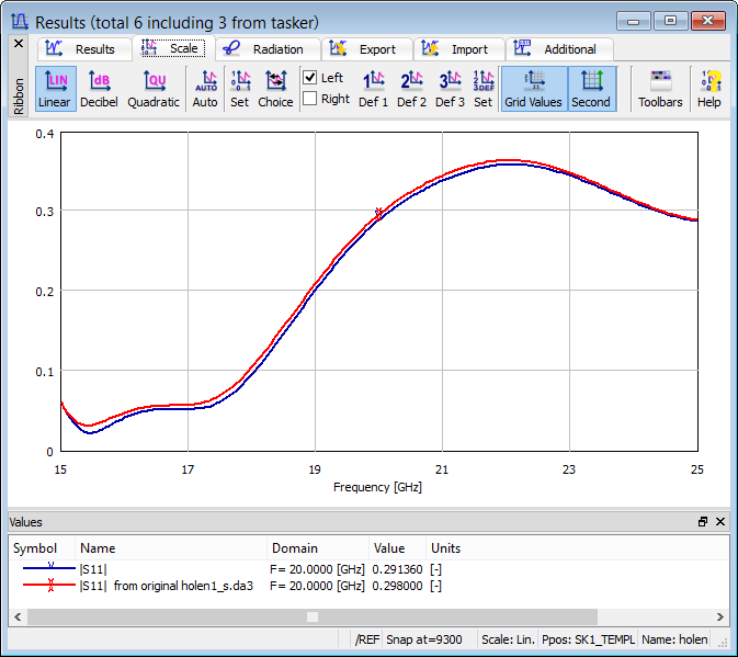
Fig. 2.10.2-12 S-parameters obtained for the antenna geometry from SAT conversion (blue) and original scenario (red).

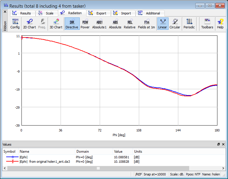
Fig. 2.10.2-13 The radiation pattern obtained for the antenna geometry from SAT conversion (blue) and original scenario (red).

If we decide to use the advanced options of SAT Filter we need to press  button (see Fig. 2.10.2-14), introduce modification to parameters and finally press  button to start the conversion process.

Let us note that on the first entry to Advanced SAT Filter parameters we have one of two available default sets of these parameters. One of two default sets can be chosen by a simple click over one of the buttons  or  available in the upper part of the dialogue. Then each of the sets can be “refined” by changing particular controls available in the lower part of the dialogues.

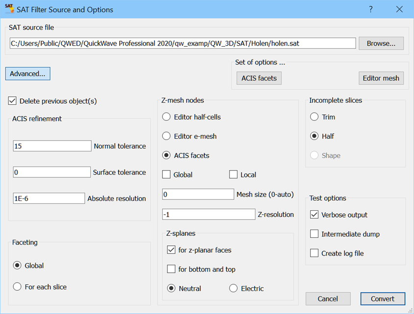
Fig. 2.10.2-14 SAT Filter advanced dialogue.

Let us explain the meaning of the SAT Filter options shown in Fig. 2.10.2-14.

·       Delete previous object(s) – a typical setting, which means that the software will delete all objects previously stored under the same name as the new object(s) to be created from *.sat file. Unchecking rarely used but may be possibly applied for duplicating converted geometry.

·       ACIS refinement group – model surfaces are approximated by planar facets with some tolerance defined by the user. For those users who are not familiar with ACIS SAT concepts we suggest to stay with default values. Possibly one can try to decrease (if necessary) Normal tolerance to get better accuracy. However slower software operation may result.

·       Faceting group – Global means that facets are created for each converted SAT body and next faceted body is sliced, For each slice creates facets for each slice.

·       Z-mesh nodes group – sets origin of z-levels used during conversion. Typically z-levels are taken from SAT file for the first pass of conversion and from QW-Editor mesh for the second pass. If for z-planar faces is checked, SAT Filter creates mesh snapping planes for the model horizontal plane surfaces. That snapping planes can be Neutral or Electric type.

·       Incomplete slices – if during conversion a slice without bottom or top appears and creation of valid element is impossible such slice can be trimmed (cut) or replaced with suspended element with height equal to half of cell Z-size.

·       Test options – check boxes for maintenance purposes.