7 Postprocessings

7.1 S-Parameters

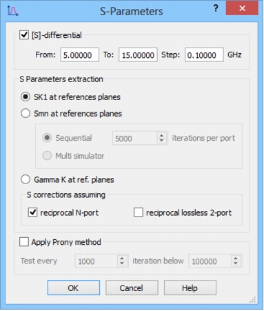
The S button in Simulation tab allows configuring the S-parameters postprocessing. Pressing that button invokes the S-Parameters postprocessing dialogue. In default setting the S-differential option is unchecked and the following options are not active. After checking S-differential checkbox, the other options become active.

In [S]-differential postprocessing we calculate the S-matrix of an N-port where N is the number of virtual ports defined in the structure. The system can include both transmission line ports and Point Ports sources/probes. For each transmission line port, the total fields at its respective reference plane are filtered through the modal template and decomposed into incident and reflected waves via the differential method. Reference impedances for S-parameter extraction are the actual frequency-dependent wave impedances of respective transmission lines. These impedances can be viewed in QW-Simulator by Setup-Switch-Extended Results option of View-S Results command. At a Point Port source/probe the [S]-differential system operates similarly as the FD-Probing. Thus for meaningful results, each Point Port source/probe should be placed between two metal elements separated by one FDTD cell. The [S]-differential system considers the port voltage (selected E-field integrated along the FDTD cell), and the current flowing into the embedding circuit (without the current component flowing into the FDTD cell). Reference impedance is taken as resistance of the Point Port source/probe, unless this resistance is zero, in which case 50 ohm is taken. Options of the [S]-differential postprocessing are described further in this Section. For detailed introduction to this postprocessing, refer to User Guide manual Section UG 2.2.1, and to other subsections of Section UG 2.2 for its examples of application to various types of transmission lines.

If choosing the option of S-parameter calculation we must decide upon the range of frequencies we are interested in, and the frequency step. The number of frequency points whereat the S-parameters are calculated increases to some extent the computing time and memory required. However, the computing time and memory used for S-parameter calculations at several hundreds of the frequency points usually does not exceed a few percent of the total computing time and memory needed to run the electromagnetic simulation. Thus the choice of this number in the range between one hundred and five hundred seems reasonable for most applications.

Note that the range of frequency in which we calculate the S-parameters cannot exceed the spectrum of the exciting pulse defined in the Ports Parameters dialogues. If this is the case, the S-parameters may be calculated with significantly increased numerical errors and QW-Simulator gives an appropriate warning.

In the S Parameters extraction frame of the S-Parameters postprocessing dialogue box we have the choice of several options:

Ÿ Sk1 at reference planes. In this case we excite the circuit only from port number 1 and calculate the incident (ak) and reflected (bk) waves at each port. This permits to calculate Sk1 = bk/a1. Note that:

The simple extraction produces results contaminated by numerical reflections from imperfect absorbing boundaries.
If the circuit is declared as reciprocal N-port, it is possible to correct the value of S11, applying the expanded formula S11=b1/a1-S12a2/a1-S13a3/a1-.... The software enforces Sk1=S1k and calculates S11=b1/a1-b2a2/a12-b3a3/a12-....
If the circuit is declared as reciprocal lossless 2-port, it is also possible to correct the value of S21, applying the formula S21=b2/a1-S22a2/a1. The software enforces |S22|=|S11| and arg(S11)+arg(S22)-2arg(S12)= ±π.

The software will not verify your declaration regarding reciprocity and losses, but it will ignore the declaration of lossless 2-port if the number of ports if different.

Ÿ Smn at reference planes. This is a general case in which we perform N simulations exciting the structure from N different ports, and then compose the complete S-matrix from N sets of partial results. Each of these sets corresponds to excitation from port i when the software calculates the parameters Ski in the same way as the parameters Sk1 are calculated in the Sk1 at reference planes postprocessing. When all N sets are available, the software corrects all the S-matrix elements for imperfect absorbing at all ports (reciprocity is irrelevant at this stage). Thus the final results of Smn calculation may somewhat differ from the N sets of partial results. There are three regimes of running the Smn at reference planes postprocessing:

In the sequential regime the software performs N consecutive simulations (with excitation from each of the N ports). Each simulation lasts for a predefined number of FDTD iterations, specified by the user in the Iterations per port box. Note that during one simulation we obtain Sk1 elements like in the Sk1 at reference planes postprocessing, and these parameters (either uncorrected or partially corrected for imperfect absorbing boundaries) are being displayed. Only after completing the N simulations with excitation from N consecutive ports QW-3D assembles the complete S-matrix, correcting all the S-matrix elements for imperfect absorbing at all port. Thus the final results of Smn calculation may be somewhat different from the intermediate results displayed during calculation.
In the Multi simulator regime, the software runs N instances of internal simulator objects in the QW-Simulator application, with a different exciting port in each of them. An apparent disadvantage of this regime resides in the increased memory requirements. However, its important advantage is the possibility of the on-line monitoring of the full corrected S-matrix, calculated for the current number of FDTD iterations. This regime works on single-processor computers; its operation on multiprocessor computers is allowed only if the QW-MultiSim option has been acquired by the user.

Ÿ Gamma K at ref. planes. It allows computing reflection coefficients Γ at several reference planes simultaneously during a single simulation run. It can be applicable when a multi-source network is considered with all the ports operating as sources simultaneously and, consequently, the scattering matrix cannot be computed.

Attention:

Only in the circuit, which is not declared to be reciprocal, the reflection coefficient is calculated independently of the outputs. In other cases it is corrected for the reflection on the output ports. In those cases any errors of analysis at the output (wrong port definition, wrong template and so on) may strongly influence also the S11 calculation.

Python code

The python code, which can be useful when creating project scripts, generated by S-Parameters dialogue for default parameters:

App.ActiveDocument.QW_PostprocessingQProny.Active = False

App.ActiveDocument.QW_PostprocessingQProny.TestEvery = 1000

App.ActiveDocument.QW_PostprocessingQProny.IterationBelow = 100000

App.ActiveDocument.QW_PostprocessingS.Active = True

App.ActiveDocument.QW_PostprocessingS.From = 5.00000

App.ActiveDocument.QW_PostprocessingS.To = 15.00000

App.ActiveDocument.QW_PostprocessingS.Step = 0.10000

App.ActiveDocument.QW_PostprocessingS.SmnType = "Sequential"

App.ActiveDocument.QW_PostprocessingS.SmnIterationsPerPort = 5000

App.ActiveDocument.QW_PostprocessingS.SParametersExtractionType = "SK1 at references planes"

App.ActiveDocument.QW_PostprocessingS.ReciprocalNport = True

App.ActiveDocument.QW_PostprocessingS.ReciprocalLossless2port = False